


Abstract
Modelling the morphology of a nova outburst provides valuable information on the shaping mechanism in operation at early stages following the outburst. We performed morpho-kinematical studies, using shape, of the evolution of the Hα line profile following the outburst of the nova KT Eridani. We applied a series of geometries in order to determine the morphology of the system. The best-fitting morphology was that of a dumbbell structure with a ratio between the major to minor axis of 4:1, with an inclination angle of 58|$^{+6}_{-7}$| deg and a maximum expansion velocity of 2800 ± 200 km s−1. Although, we found that it is possible to define the overall structure of the system, the radial density profile of the ejecta is much more difficult to disentangle. Furthermore, morphology implied here may also be consistent with the presence of an evolved secondary as suggested by various authors.
1 INTRODUCTION
A classical nova outburst occurs on the surface of a white dwarf (WD, the primary) following extensive accretion from a secondary star (typically a late-type main-sequence star that fills its Roche lobe; Crawford & Kraft 1956). This outburst, a thermonuclear runaway, ejects ∼10−6–10−4 M⊙ of matter from the WD surface with velocities from hundreds to thousands of km s−1 (see, e.g. Bode & Evans 2008; Bode 2010, and references therein). Nova outbursts can be divided into classical novae and recurrent novae (RNe). As the latter name suggests, this outburst usually occurs on time-scales of the order of tens of years and the majority are observed to have evolved secondaries (e.g. Darnley et al. 2012). Such a short recurrence time-scale is usually attributed to a high-mass WD, probably close to the Chandrasekhar limit, together with a high accretion rate (Starrfield, Sparks & Truran 1985; Yaron et al. 2005).
Nova Eridani 2009 (hereafter, KT Eri) was discovered on 2009 November 25.54 ut in outburst by Itagaki (2009). Low-resolution optical spectra obtained on 2009 November 26.56 showed broad Balmer series, He i 5016 Å and N iii 4640 Å emission lines with full width at half-maximum of Hα emission around 3400 km s−1 (Maehara & Fujii 2009). This object was confirmed later as an ‘He/N’ nova (Rudy et al. 2009).
The discovery date was not the date of outburst. Other authors suggested that the nova was clearly seen in outburst on 2009 November 18 and that the outburst occurred after 2009 November 10.41 (Drake et al. 2009). Hounsell et al. (2010) searched the Solar Mass Ejection Imager (SMEI) archive and the Liverpool Telescope SkyCamT observations and found KT Eri clearly in outburst on 2009 November 13.12 ut with a pre-maximum halt occurring on 2009 November 13.83. They found the outburst peak to have occurred on 2009 November 14.67 ± 0.04 ut (which is taken as t = 0) with magnitude mSMEI = 5.42 ± 0.02. Furthermore, Hounsell et al. (2010) show KT Eri to be a very fast nova with t2 = 6.6 d (the time taken for the magnitude to decline by two magnitudes from optical peak). A distance to the system has been derived by Ragan et al. (2009) as 6.5 kpc. However, it is noteworthy that they assumed that t2 = 8 d which is slightly different from that derived by Hounsell et al. (2010) (although the SMEI magnitudes are white light effectively and the t2 would be expected to differ from that in V for example).
KT Eri has also been detected at radio wavelengths (O’Brien et al. 2010) and as an X-ray source (Bode et al. 2010). The Swift satellite's first detection of KT Eri with the X-ray Telescope was on day 39.8 after outburst as a hard source (Bode et al. 2010). This was also the case on day 47.5. However, by day 55.4 the supersoft source (SSS) phase emerged (the dates have been corrected to the t = 0 given above). On day 65.6 the SSS softened dramatically. Bode et al. (2010) also noted that the time-scale for emergence of the SSS was very similar to that in the RN LMC 2009a (Bode et al. 2009).
An archival search for a previous outburst was carried out with the Harvard College Observatory plates by Jurdana-Šepić et al. (2012), where they identified the progenitor system. However, no previous outburst was observed. They found a periodicity of 737 d which was attributed to reflection effects or eclipses in the central binary. A shorter periodicity of 56.7 d was also found by Hung, Chen & Walter (2011) which was attributed to arise from the hotspot on the WD accretion disc although Jurdana-Šepić et al. (2012) find no evidence to support the shorter frequency. Jurdana-Šepić et al. (2012) also derive a quiescent magnitude 〈B〉 = 14.7 ± 0.4, which combined with the periodicity above suggests that the secondary star is evolved and likely in, or ascending, the red giant branch. This result is corroborated by Darnley et al. (2012) and Imamura & Tanabe (2012). Furthermore, Jurdana-Šepić et al. (2012) predict that if KT Eri is an RN then it should have a recurrence time-scale of centuries.
In this paper, we present morpho-kinematical modelling, using shape1 (Steffen et al. 2011), of the evolution of the Hα line profile. In Section 2, we present our observational data; in Section 3, we present the modelling procedures and the results are presented in Section 4. Finally, in Section 5 we discuss the results and present our conclusions.
2 OBSERVATIONS
Optical spectra of KT Eri were obtained (Table 1) with the Fibre-fed Robotic Dual-beam Optical Spectrograph (FRODOSpec; Morales-Rueda et al. 2004), a multipurpose integral-field input spectrograph on the robotic 2 m Liverpool Telescope (Steele et al. 2004). The dual beam provides wavelength coverage from 3900 to 5700 Å (blue arm) and 5800 to 9400 Å (red arm) for the lower resolution (R = 2600 and 2200, respectively), and 3900 to 5100 Å (blue arm) and 5900 to 8000 Å (red arm) for the higher resolution (R = 5500 and 5300, respectively).
Log of optical spectral observations of KT Eri with the FRODOSpec instrument on the Liverpool Telescope.
| Date | Days after | Exposure |
|---|---|---|
| outburst | time (s) | |
| 2009 Dec. 26 | 42.29 | 60 |
| 2009 Dec. 30 | 46.25 | 60 |
| 2009 Dec. 31 | 47.20 | 60 |
| 2010 Jan. 01 | 48.16 | 60 |
| 2010 Jan. 02 | 49.15 | 60 |
| 2010 Jan. 03 | 50.15 | 60 |
| 2010 Jan. 04 | 51.15 | 60 |
| 2010 Jan. 07 | 54.20 | 60 |
| 2010 Jan. 11 | 58.16 | 60 |
| 2010 Jan. 12 | 59.14 | 60 |
| 2010 Jan. 14 | 61.14 | 60 |
| 2010 Jan. 16 | 63.13 | 60 |
| 2010 Jan. 20 | 67.26 | 60 |
| 2010 Jan. 25 | 72.20 | 60 |
| 2010 Jan. 26 | 73.13 | 60 |
Data reduction for FRODOSpec was performed through two pipelines. The first pipeline reduces the raw data. This includes bias subtraction, trimming of the overscan regions and flat fielding. Then the second pipeline performs a series of operations on the data, including flux extraction, arc fitting, throughput correction, linear wavelength rebinning and also sky subtraction (Barnsley, Smith & Steele 2012). Any absorption features were patched over and then using the Starlink Figaro IRFLUX task, correction for the instrumental efficiency/atmospheric transmission and relative flux calibration was performed on the KT Eri spectra using the standard star HD19445. Fig. 1 shows the evolution of the Hα emission. The full spectra will be shown in a forthcoming paper.
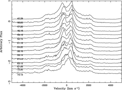
Hα emission-line evolution. Numbers on the left are days post-outburst.
3 MODELLING
Work by Hutchings (1972), Solf (1983), Slavin, O’Brien & Dunlop (1995), Gill & O’Brien (2000) and Harman & O’Brien (2003), resolved nova shells with optical imaging which showed a myriad of structures. Several mechanisms for the formation of these structures were put forward. These included a common envelope phase during outburst, the presence of a magnetized WD and an asymmetric thermonuclear runaway (for a recent review see O’Brien & Bode 2008). The most widely accepted shaping mechanism is that involving a common envelope phase.
Previous works, e.g. Munari et al. (2011, hereafter MRB11) and Ribeiro et al. (2011, hereafter RDB11), have extensively described the modelling procedures we use here and built a large grid of early outburst synthetic spectra. These synthetic spectra were derived from the following structures: (i) polar blobs with an equatorial ring, (ii) a dumbbell structure with an hourglass overdensity, (iii) a prolate structure with an equatorial ring, (iv) a prolate structure with tropical rings and (v) a prolate structure with polar blobs and an equatorial ring. For each of the structures, the parameter space, between 0°and 90°for the inclination angle (where an inclination i = 90° corresponds to the orbital plane being edge-on, and i = 0° being face-on), and 100 and 8000 km s−1 for the maximum expansion velocity, was explored to retrieve a synthetic spectrum for each set of parameter combinations. The synthetic spectra were then compared with the observed spectra and the flux was matched via χ2 minimization.
Here, we have also explored the optimizer module within shape. This allows us to automatically improve the fit of a set of parameters using a least-squares minimization technique. Here, we estimate an initial structure, velocity field (in order to retrieve a 1D line profile) and/or other parameters. The general strategy to optimize a structure is to choose one or more of the parameters to optimize. We then provide a range of values which the optimizer searches around. In general, they are the same as those described above for inclination and maximum expansion velocity. These are taken as initial guesses by the module. Then, in case of this study, a line profile is loaded which drives the minimization process.
Once the optimization process starts, the model is compared with the observation to generate a least-squares difference. The values of the parameters are varied over the range that was pre-set to find the least-squares solution and in the order they appear in the stack. The cycle of optimization is repeated until a minimum difference is achieved.
This technique allows shape to find the best-fitting results for the structure described above. The parameters that were allowed to be optimized were the inclination and maximum expansion velocity. Allowing for more parameters to vary is not advisable and might produce unrealistic models. However, this technique does not provide uncertainty estimates on the parameters at the time of writing this paper.
Applying the synthetic spectra derived from the structures described above to the observed spectra on day 42.29 following outburst did not provide a good fit to the observations (as an example, in Fig. 2, we show the best-fitting result for a prolate structure with an equatorial ring). This is unsurprising due to the fact that the spectrum observed here is at a much later date than those in MRB11 and RDB11 (although in the latter case the structure was also evolved to a much later date). In particular RDB11, were able to demonstrate that when the early models (which were volume filled) were evolved to a much later date (in this case a thin shell), this appeared to replicate well the effect of the termination of the post-outburst wind phase and complete ejection of the envelope (della Valle et al. 2002).
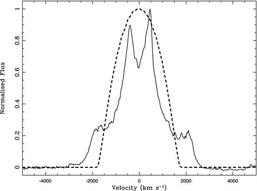
Best-fitting synthetic spectra (dashed line), for a prolate structure with an equatorial ring, to the observed spectra (solid line) on day 42.29 following outburst.
As KT Eri is suggested to harbour an evolved secondary (Jurdana-Šepić et al. 2012), we explored a structure similar to RS Ophiuchi (Fig. 3, see also Ribeiro et al. 2009). However, as mentioned in Jurdana-Šepić et al. (2012) the secondary in KT Eri may not be as evolved as in RS Oph. This suggests that there is not as strong a wind from the secondary pre-outburst, which may be associated with the origin of the central overdensity modelled in RS Oph.
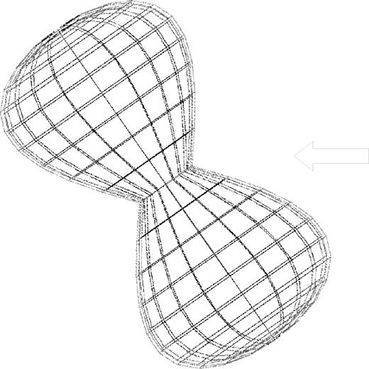
KT Eri's model mesh, as the input geometry, as visualized in shape. The inclination of the system is defined as the angle between the plane of the sky and the central binary system's orbital plane. The arrow indicates the observer's direction.
The bipolar structure was assumed to have a ratio of the major to minor axis of 4:1. This was suggested by the ratio of the broad wing width to the central double peak separation being in this ratio (Fig. 1).
We further applied a radial density profile which varied as 1/r (where r is the radial distance away from the centre of the outburst). This was investigated via multiple trial and error on the radial density profile, using the optimization module, to see what the best fit to the observed spectrum was, before exploring in more detail the parameter space of interest. The first spectrum explored was that of day 42.29 after outburst and then the best-fitting parameters found were applied to day 63.13 after outburst, always keeping the parameters for the inclination and maximum expansion velocity the same.
As with previous work, apart from Ribeiro et al. (2009), to retrieve the synthetic line profiles we used the Mesh Renderer, which directly used the 3D mesh structure (Fig. 3) and transfers it to a regular 3D grid. Along with the spatial distribution of the mesh, the physical properties that depend on position in space are transferred to the grid. These were the velocity, inclination and density. In the Mesh Renderer the emissivity, used to create the synthetic line profiles, is proportional to the density squared.
4 RESULTS
4.1 Early epoch observations (t = 42.29 d)
The results of exploring the full parameter space are shown in Fig. 4. The best-fitting result implies an inclination of i = 58|$^{+6}_{-7}$| deg and a maximum expansion velocity of Vexp = 2800 ± 200 km s−1. In comparison, adopting the optimizer technique, the best-fitting result suggests an inclination i = 55° and Vexp = 2800 km s−1 (Fig. 5), i.e. well within the uncertainty estimates of exploring the full parameter space.
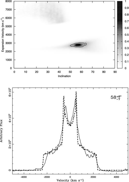
Best-fitting model results and comparison between the observed and model spectrum (day 42.29 after outburst) using the techniques described in MRB11 and RDB11. Top – derivation of the most likely result for the structure, where the grey-scale represents the probability that the observed |$\mathcal {X}^2$| value is correct. The solid line represents the 1σ boundary. Furthermore, the island at the high-velocity end is due to the finite resolution of the model (for a brief discussion see Ribeiro 2011). Bottom – the observed (solid black) and synthetic (dashed black) spectra for the best-fitting inclination, shown in the top-right-hand corner, with its respective 1σ errors.
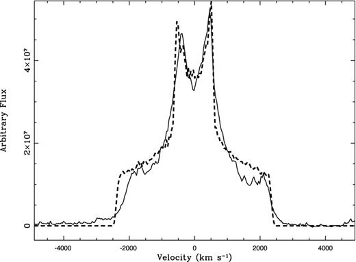
Best-fitting result using the optimizer module technique assuming a 1/r density distribution. The observed (solid black, t = 42.29 d) and synthetic (dashed black) spectra are compared. The results suggest an inclination of 55° and Vexp = 2800 km s−1.
The very similar results derived using the two methods allow us to very quickly explore different structures and find a best fit to the observed data using the optimizer technique. Considering the much reduced computational time that the optimizer technique allows for, we are able to explore other parameters efficiently. For example, in an attempt to see the effects of changing the radial density profile, we changed this parameter so that it varied as 1/r2 and also assuming a constant density throughout (Fig. 6). The results suggest an inclination of 51° and 64°, and maximum expansion velocities of 3000 km s−1 and 2600 km s−1 for a 1/r2 and constant density profile, respectively. Fig. 6 shows that these two assumptions for the density were not optimum fits to the observed spectra, either overpredictiing or underpredicting the fluxes in different parts of the spectrum. Therefore, the derived best-fitting density profile is assumed to be that of a 1/r distribution. However, the results for 1/r2 and a constant density profile are within the error bars derived for the 1/r fit.
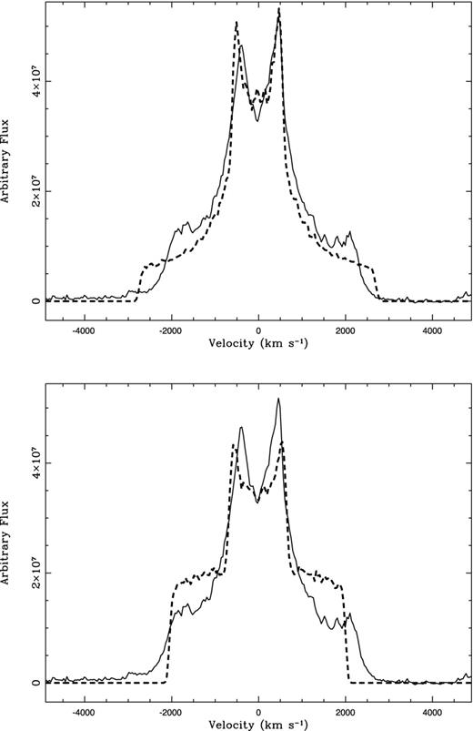
Best-fitting results using the optimizer module technique for the earlier epoch observations (t = 42.29 d). Top – assuming a 1/r2 radial density distribution, the results suggest an inclination of 51° and Vexp = 3000 km s−1. Bottom – assuming a constant density distribution, the results suggest an inclination of 64° and Vexp = 2600 km s−1. The observed (solid black) and synthetic (dashed black) spectra are compared.
The degeneracy between our assumed structure and density profiles does not permit us to say with a degree of certainty which are the best-fitting density profiles; in all cases, the structure reproduces the overall shape of the synthetic spectrum. Other effects, which are not taken into account in the modelling, that may change the shape of the line profile, include the consideration of self-absorption by the Hα line, which in our models is assumed to be optically thin, but is consistent for example, with the fact that we observe structures in the line profiles that are to a large extent symmetrical.
4.2 Later observations (t = 63.13 d)
Taking the values for the inclination and maximum expansion velocity from the previous subsection, both 1/r and 1/r2 density profiles were applied to the later epoch observations (Fig. 7). Inspection of Fig. 7 would suggest that the profile resulted from a 1/r2 density profile would be the better fit. However, the modelling of this line is complicated by the fact that there is an evolution of the line profile shape (Fig. 1). This evolution was discussed in Ribeiro (2011), who suggested that as the soft X-rays emerge, sampling nuclear burning on the surface of the WD, the Hα emission arising from the ejecta may be contaminated by emission close to the central binary.
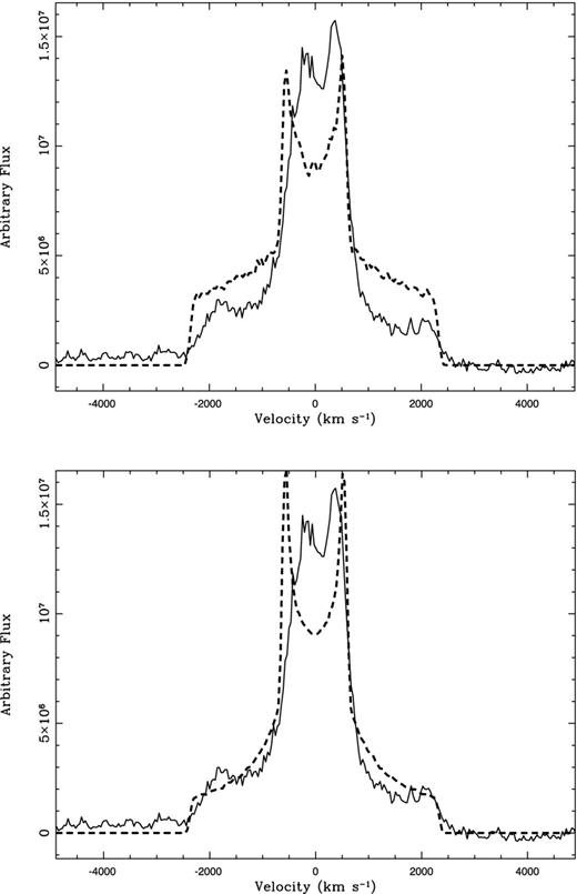
Best-fitting results for the later epoch observations (t = 63.13) using the optimizer module technique assuming a 1/r (top) and 1/r2 (bottom) density profiles. The observed (solid black) and synthetic (dashed black) spectra are compared.
5 DISCUSSION AND CONCLUSIONS
The observed Hα line profile from KT Eri on day 42.29 is modelled with a dumbbell shaped expanding nebulosity (Fig. 3) assuming a 1/r radial density profile, Vexp = 2800 ± 200 km s−1 and inclination angle of 58|$^{+6}_{-7}$| deg as the best-fitting parameters. It is noteworthy that at this time the line profile we observe is likely to be due to the Hα emission as the spectra in Ribeiro (2011) do not show any contribution from [N ii] emission which played a role in the line shape of V2491 Cygni (RDB11).
The later epoch line profile (day 63.13) was also modelled but this time the best fit resulted from a 1/r2 density profile. However, caution should be exercised here. Ribeiro (2011) described the evolution of the Hα emission line, which showed the central regions of the line gain in intensity compared with the whole profile. This was interpreted as arising from material closer to the WD as the ejecta become optically thin and/or diffusion of the outer faster moving material. Similarly, evidence for emission by material closer to the WD may be supported by the relationship between the emergence of He ii 4686 Å and the SSS (Ribeiro 2011).
Earlier spectra than those shown here showed that the line profile appears to be asymmetric with respect to the rest wavelength (Ribeiro 2011). This may be a combination of the systemic velocity of the system and/or the associated termination of the post-outburst wind phase, which happens during the first few weeks following the nova outburst (e.g. Hachisu et al. 2000), and complete ejection of the envelope (della Valle et al. 2002; RDB11), or optical depth effects.
What is certainly true with this type of study is that caution should be exercised when assuming a morphology arising from line profiles without the aid of imaging to constrain the models. Previous work dealt with modelling soon after the outburst, where most of the ejecta contribute to the line profile, and hence a constant density profile can be assumed; while at later stages although the morphology of the system will be the same, the main contributor to the line profile may be a combination of ejecta and ultraviolet illumination of the ejecta by the central source. This may be implied by the narrowing of the central peaks as shown in Fig. 7 compared with Fig. 6. However, we cannot also rule out the fact that the higher velocity material will decrease in density faster as the ejected shell expands outward.
The structure and inclination angle derived here are consistent with those inferred by Jurdana-Šepić et al. (2012). The inferred structure is also similar to that derived for RS Oph (Ribeiro et al. 2009). Here, mass-loss between outbursts from the red giant secondary star of the binary leads to an enhanced pre-outburst density in the binary equatorial plane external to the binary system itself. Hydrodynamic simulations by Mohamed & Podsiadlowski (2012) and Mohamed, Booth & Podsiadlowski (2013) then produce the bipolar structures observed in the ejecta. In KT Eri, the secondary star is thought to be a low-luminosity giant and hence the mass of any pre-outburst envelope may be less than that in RS Oph. We also note however that there was no direct evidence of interaction with pre-existing material (e.g. through hard X-ray emission similar to that in RS Oph; Bode et al. 2006, although the lower density of any pre-existing wind in KT Eri and the object's factor ∼4 greater distance than RS Oph would have made such emission less detectable in this case).
The authors are grateful to W. Steffen and N. Koning for valuable discussion on the use of shape. VARMR acknowledges financial support from the Royal Astronomical Society through various travel grants. The South African SKA Project is acknowledged for funding the post-doctoral fellowship position at the University of Cape Town. RMB was funded by an STFC studentship. We thank an anonymous referee for valuable comments on the original manuscript.
South African Square Kilometre Array Fellow.
Available from http://bufadora.astrosen.unam.mx/shape/index.html
