Light bosons in the photosphere and the solar abundance problem

Abstract

INTRODUCTION

Agreement between predictions of solar interior models and helioseismological measurements has deteriorated in recent years, due to a downwards revision in standard solar abundances. Recent photospheric analyses (Allende Prieto, Lambert & Asplund 2001, 2002; Asplund et al. 2004, 2005b, 2009; Asplund, Grevesse & Sauval 2005a; Scott et al. 2006, 2009; Meléndez & Asplund 2008) have indicated that the solar metallicity is about 20 per cent lower than previously thought (Grevesse & Sauval 1998). In particular, the current reference photospheric abundances (Asplund et al. 2009) of the important elements C, N and O are smaller than the previous reference values (Grevesse & Sauval 1998) by 0.09, 0.09 and 0.14 dex, respectively. Standard solar models computed with the revised surface metal abundances show large discrepancies with the depth of the convection zone, the surface helium abundance and the sound speed profile inferred from helioseismology (Basu & Antia 2004, 2008; Bahcall et al. 2005a; Bahcall, Serenelli & Basu 2006; Yang & Bi 2007; Serenelli et al. 2009). This has been variously referred to as ‘the solar model(ling) problem’ (Drake & Testa 2005; Asplund 2008; Morel & Butler 2008), ‘the solar oxygen crisis’ (Ayres, Plymate & Keller 2006; Socas-Navarro & Norton 2007; Ayres 2008) or ‘the solar abundance problem’ (Guzik & Mussack 2010; Serenelli, Haxton & Peña-Garay 2011).

The most common approaches to the solar abundance problem to date have been to recheck the photospheric abundances (Drake & Testa 2005; Ayres et al. 2006; Ayres 2008; Caffau et al. 2008, 2010; Centeno & Socas-Navarro 2008; Morel & Butler 2008), or to modify solar models in an attempt to accommodate both the measured abundances and data from helioseismology. Efforts in the latter category have included enhanced diffusion (Guzik, Watson & Cox 2005), late-stage accretion of low-metallicity gas (Guzik et al. 2005; Castro, Vauclair & Richard 2007; Guzik & Mussack 2010; Serenelli et al. 2011), modifications of opacities (Badnell et al. 2005; Bahcall, Serenelli & Basu 2005b; Christensen-Dalsgaard et al. 2009), internal gravity waves (Arnett, Meakin & Young 2005; Charbonnel & Talon 2005) and enhanced energy transport in the solar core due to gravitational capture and scattering of dark matter (Cumberbatch et al. 2010; Frandsen & Sarkar 2010; Taoso et al. 2010). Despite nearly a decade of effort (and a few errant claims to the contrary), none of these approaches has proven successful in solving the problem.

Here, we propose an alternative approach: examining effects of new physics on the measurement of solar photospheric abundances. Specifically, we investigate the impact on derived elemental abundances of mixing between photons and new light bosons, such as axions, in the line-forming regions of the photosphere.¹

The equivalent width of a spectral line is defined as the width in wavelength space of a rectangle having the same area as the integrated region between the line and the continuum (where the height of the rectangle is given by the continuum level). Equivalent width is a relative measure of line strength, and depends not only on the abundance of a given element, but also on the attenuation of the total continuum as it passes through the line-forming region. For this reason, both line and continuum fluxes must be carefully calculated with radiative transfer simulations before elemental abundances can be inferred. If additional plasma effects in the photosphere enhance continuum photon attenuation via oscillation into light bosons such as axions, then the equivalent width of absorption lines used to calculate elemental abundances would be suppressed. By combining the axion conversion effect with earlier radiative transfer calculations, we will show how this could occur in principle, and assess whether this effect could arise from existing particle theories in such a way as to solve the solar abundance problem.

The PQ mechanism in QCD is not the only possible origin of such a particle, however. Axion-like particles (ALPs) are a ubiquitous element in string theory compactifications (Svrcek & Witten 2006; Dasgupta, Firouzjahi & Gwyn 2008), in which the moduli describing the compact extra dimensions can appear to observers as internal U(1) gauge degrees of freedom. More generally, U(1) symmetries appear in many high-energy extensions of the SM, giving rise to exotic particles with interactions similar to the axion. Like axions, ALPs interact with photons via a term of the form as in equation (3). Unlike axions, they do not necessarily solve the strong CP problem, nor require such small couplings or m_a ∝ 1/g_aγ.

We begin by showing in Section 2 how photon–ALP oscillation can affect the linear attenuation coefficient – and hence the equivalent width of an absorption line – in the solar atmosphere at optical depths τ < 1. We demonstrate in Section 3 that with a large enough coupling g_aγ, a low-mass particle with a term like equation (3) could affect the solar atmosphere enough to modify absorption lines in an observable way. As we discuss in Section 4, however, the coupling strength required to produce such an effect is much larger than the coupling allowed by current experimental bounds on standard ALPs. We go on to show that this rules out not only ALPs as photospheric solutions to the solar abundance problem, but also hidden photons and chameleons. We conclude in Section 5 that unless some other light boson with an axion-like or similar kinetic-mixing-type coupling to the photon can be found that somehow evades the existing experimental constraints, the solar abundance problem cannot be solved by light bosons in the photosphere.

THEORY

Changing inferred abundances

Photon–ALP conversion in the solar atmosphere

Conversion in plasma fields

Conversion in a bulk magnetic field

Figure 1.

Open in new tabDownload slide

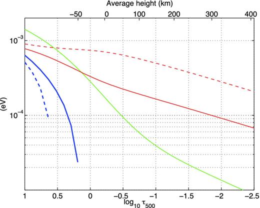
Green: average plasma frequency ω_pl (eV) as a function of optical depth at 500 nm (bottom axis) and averaged height (upper axis) in a convection simulation of the Solar atmosphere. Red: gas contribution to Δ_||, plotted as |$(\omega \Delta _{||}^{\rm gas})^{1/2}$| at photon energies corresponding to λ = 300 nm (dashed – primarily neutral hydrogen) and 900 nm (solid – primarily electrons). When the difference between the plasma and gas quantities (thick blue lines) is positive, |$\omega _{\rm pl}^2 - \omega \Delta _{||}^{\mathrm{gas}} > 0$|⁠, resonant enhancement may occur. The value of this difference at a given height corresponds to the ALP mass m_a for which resonant conversion takes place.

Equation (11) describes a Lorentzian (Breit–Wigner) distribution in Δ_a ∝ 1/ω modulated by the sin ² term, with resonance at the plasma frequency and width Δ_aγ ∝ B. When Δ_|| − Δ_a goes to zero, photon conversion to ALPs is enhanced. We later show that for m_a ∼ 10⁻⁵–10⁻³ eV, this has the potential to occur in the region of the solar atmosphere where line formation occurs. The plasma frequency ω_pl increases quickly with increasing optical depth. Given the |$\omega _{\rm pl}^{-4}$| suppression of equation (11), this means that conversion is highly suppressed at depths below the resonance depth h_res. There are thus three qualitatively different regions in the solar atmosphere: (1) below h_res, the denominator of P₀ is dominated by the plasma term |$\Delta _{\rm pl}^2 \propto \omega _{\rm pl}^{4}$|⁠, ensuring that very little conversion occurs below the resonance height; (2) at h_res, Δ_pl ≃ Δ_a and resonance occurs: conversion is enhanced and P₀ → 1 for a small region; and (3) above h_res, P₀ becomes approximately constant as the plasma frequency falls and the constant term Δ_a essentially dominates Δ_osc, providing moderate conversion rates. The existence of region (2) is contingent on the plasma effects being larger than the contribution from neutral gas; otherwise, Δ_|| and −Δ_a are always positive, prohibiting cancellation.

We point out that many references (e.g. Raffelt 1988; Mirizzi et al. 2008) do not include |$\Delta _{||}^{\rm {gas}}$|⁠. This is because in situations such as hot stellar interiors or the interstellar medium, the ionization fraction is so large that |$\Delta _{||}^{\rm {gas}}$| is always subdominant to Δ_pl. Indeed, the intermediate temperatures encountered in the solar atmosphere make it one of the few places where both the gas refractive index and plasma frequency contribute to similar degrees. Fig. 1 illustrates these effects, showing that resonant conversion may only occur below log τ ∼ 0 (i.e. at larger optical depths). The blue lines show the ALP mass at which resonant conversion may occur for two different photon wavelengths.

EFFECTS ON SOLAR ABUNDANCES

To determine the impact of photon–ALP conversion in the photosphere on solar abundances, we calculated the expected correction factor Δlog ϵ (equation 7) using the 3D hydrodynamic solar model atmosphere from Asplund et al. (2009). We computed the ALP-induced opacity |$\kappa ^a_\lambda$| at wavelengths from 300 to 1000 nm, at each point in an (x, y, z) grid with resolution 50 × 50 × 500, sampled from the atmosphere simulation. Our extracted grid covers 6 × 6 Mm, in the horizontal directions, and optical depths in the range −3 ≤ log τ ≤ 0.5, in which the majority of line formation occurs and below which conversion is negligible. We did this for 90 snapshots from the simulation, corresponding to 45 min in solar time before averaging. All averages presented here are carried out over time and over the undulating surfaces of particular optical depths to give averages on the τ₅₀₀-scale. We averaged the local values of |$\kappa ^a_\lambda$| over (x, y, t) slices of common optical depth at 500 nm, to arrive at expected abundance corrections as a function of wavelength and formation height of arbitrary spectral lines. Spatial and temporal changes in line profiles due to convective motions occur over the length-scales and lifetimes of convective granules, which are approximately 1 Mm and 10 min for the Sun (Stein & Nordlund 1998; Asplund 2005). As these scales are significantly smaller than the extent of the simulation, our averaged values should accurately represent the expected effect of ALPs on the mean solar spectrum.

The continuum opacities include bound–free absorption by the first three ionization stages of 15 of the most abundant elements, as computed by the Opacity Project and the Iron Project (Badnell et al. 2005). The absorption by the anions of H, He, C, N and O is also included, as well as that by the molecules H₂, H|$_2^+$|⁠, H|$_2^-$|⁠, OH, CH, H₂O and CO⁻ and the pressure induced absorption of transient (H i+H i)-, (H i+He i)-, (H₂+H i)-, (H₂+He i)- and (H₂+H₂) pairs. A complete list with detailed references was presented by Hayek et al. (2010). The opacity in the 380–1644 nm range is dominated by the bound–free absorption by H⁻, by free–free absorption of H i and H⁻ further into the infrared and by bound–free absorption by H i and various metals further into the ultraviolet.

Depending on initial conditions and simulation details, magnetohydrodynamic models of the photosphere predict vertical magnetic field amplitudes in the quiet Sun up to 0.1 T, with domains ranging from a few hundred to 1000 km in diameter at line-forming heights (Stein & Nordlund 2006; Cheung & Cameron 2012; Moll, Cameron & Schussler 2012). This means that equation (18) is valid for all our calculations; if s were equal to or smaller than the scaleheight H_κ, equation (24) would be needed instead. The horizontal component of the magnetic field can furthermore be two to five times larger than the vertical component (Steiner et al. 2009). We therefore take 〈B〉 = 0.1 T, but caution that some studies (including Steiner et al. 2009) favour a more modest 0.001–0.01 T.

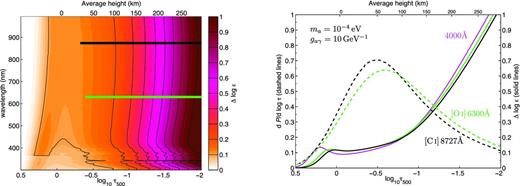
Using a coupling that is only mildly in tension with current constraints (see Section 4.1), g_aγ = 10⁻⁷ GeV⁻¹, we find that resonant photon–axion conversion has very little impact on the effective opacity: Δlog ϵ < 10⁻¹¹. This is many orders of magnitude below what is required to solve the solar abundance problem. We illustrate the impact of resonant photon–axion conversion on the effective line opacity in Fig. 2 with m_a = 10⁻⁴ eV and a very large value of g_aγ = 0.1 GeV⁻¹, giving resonant conversion at a mean optical depth of log 〈τ〉 ∼ 0.2. We also show the contribution functions for the 630.0 nm [O i] and 872.7 nm [C i] forbidden lines (reproduced from 3D line formation calculations presented by Caffau et al. (2008) and Caffau et al. (2010), respectively), indicating the contributions from different atmospheric heights to the formation of these lines. These two lines are important contributors to the determination of oxygen and carbon abundances (Allende Prieto et al. 2001, 2002; Asplund et al. 2004, 2005b, 2009). Due to the |$\Delta _{||}^{\rm {gas}}$| contribution, which may be seen as a suppression of the effective photon mass by the index of refraction of neutral hydrogen, resonant conversion within most of the line-forming region is disallowed. We note the sharp rise at low optical depths is because of the sharp drop in the opacity at these heights: Fig. 2(b) shows the relative change in line strength, reflecting the decrease in continuum opacity; the absolute change at optical depths less than ∼−2 has no observable effect.

Figure 2.

Open in new tabDownload slide

The effect of resonant photon–axion conversion on the effective line widths. Left: abundance correction effect in the solar atmosphere due to particles with an axion-like coupling, as a function of optical depth τ and wavelength. Here, m_a = 10⁻⁴ eV and we have set g_aγ = 0.1 GeV⁻¹, to illustrate the effect, although the allowed value of g_aγ by observational searches is much lower. Horizontal bars indicate the central 68 per cent intervals of the line formation contribution functions for the 630.0 nm [O i] (green) and 872.7 nm [C i] (black) forbidden neutral atomic lines. Right: constant-wavelength slices through the left-hand panel for (solid lines) λ = 400 nm (magenta), 630 nm (green) and 875 nm (black). The peaks are due to resonant photon–ALP conversion near optical depth log 〈τ〉 = 0. The green and black dashed lines represent the contribution functions dP/dlog τ to the 630.0 nm [O i] and 872.7 nm [C i] absorption lines, respectively. In both cases, ∫dP = 1 with τ being the monochromatic optical depth at the central wavelength of the respective absorption line (rather than τ₅₀₀).

If the coupling g_aγ is pushed to even larger values g_aγ > 10 GeV⁻¹, non-resonant conversion can provide corrections of Δlog ϵ > 0.2 dex in the centre of the region of line formation. We illustrate this in Fig. 3. Taken naively, the correction factors we present here could offer at least a partial solution to the solar abundance problem, as abundances from all lines would increase relative to their expected values. This example combination of m_a and g_aγ would induce the necessary 0.1–0.2 dex change in abundances from some common C and O indicators; similar effects would be expected with other lines used for abundance determination, as they typically form at similar optical depths. The exact amount by which the abundance inferred from each line and species would rise would depend on line choice, line-to-line differences in wavelengths and formation depths, the magnetic field structure and so on.

Figure 3.

Open in new tabDownload slide

The effect of photon–axion conversion above the resonance region, with a coupling large enough to solve the solar abundance problem. m_a = 1 × 10⁻⁴ eV as in Fig. 2, but g_aγ = 10 GeV⁻¹. The solid lines on right-hand figure are for λ = 400 nm (magenta), 630 nm (green) and 875 nm (black); the dashed lines represent the O i and C i contribution functions (see Fig. 2 caption). The conversion probability remains constant throughout the line-forming region of the atmosphere, and the rise in Δlog ϵ is due to the falling bulk opacity with height. We note that the extremely large coupling required is ruled out by several orders of magnitude.

However, to this point we have not carefully considered the viability of the couplings required, in view of independent constraints from solar core or laboratory searches for axions and ALPs. In the following section, we discuss those bounds and the possibility of achieving this effect with real particle models, showing that any observable effect is in fact already ruled out by existing bounds on ALPs.

DISCUSSION

ALPs

There are three types of photon–ALP conversions that can be probed in order to constrain g_aγ and m_a.³

• Conversion in hot dense cores of stars should produce X-ray energy ALPs. Observations of horizontal branch stars constrain the rate of energy loss during their He-burning phase (Raffelt 1999). The Sun itself would lose significant amounts of energy from its core if standard ALPs with couplings large enough to solve the solar abundance problem truly existed, giving rise to observable effects in the frequencies of p-mode (sound wave) oscillations (Schlattl, Weiss & Raffelt 1999) and the solar neutrino flux (Gondolo & Raffelt 2009). Conversion in the Sun can also be directly probed: pointing an ‘axion helioscope’ at the Sun give strict limits on the reconversion of ALPs into X-rays (Arik et al. 2009). The CERN Axion Solar Telescope bound on Solar core ALP production and reconversion is g_aγ < 9 × 10⁻¹¹ GeV⁻¹ for masses less than 10⁻² eV.

• Light shining through wall (LSW) experiments probe reconversion of ALPs produced from laser beams in an intense magnetic field. Current bounds are from the any light particle search (ALPS; Ehret et al. 2010) and GammeV (Chou et al. 2008) experiments. Both shine a high-intensity 532 nm laser beam at a stopper in a transverse magnetic field, and set bounds based on the (non) observation of reconverted photons behind the stopper. For masses below 1 meV, the ALPS bound is g_aγ ≲ 6 × 10⁻⁸ GeV⁻¹ whereas the GammeV bound is g_aγ ≲ 3 × 10⁻⁷ GeV⁻¹.

• Vacuum polarization changes from ALP conversion of a linearly polarized infrared laser beam in a 2.3 T magnetic field has been probed by the polarizzazione del vuoto con laser (PVLAS) experiment (Bregant et al. 2008). Vacuum dichroism occurs when some of the photons oscillate into ALPs, causing a loss of part of the beam with polarization parallel to the magnetic field, and thus cause a small beam rotation. Conversely, birefringence occurs when ALP oscillation causes a phase lag of one of the polarization components, causing an ellipticity to develop in the beam polarization. The strongest bound to date from this effect has been provided by the dichroism limits of PVLAS: g_aγ ≲ 4 × 10⁻⁷ GeV⁻¹ for ALP masses below ∼1 meV.

These limits are much too strong to allow standard axions or ALPs to produce an observable effect in the solar atmosphere. Nonetheless, there are classes of models in which some of these bounds do not apply. It was pointed out by Masso & Redondo (2005) that if the ALP is a composite object analogous to the neutral pion, then the photon-ALP conversion can be suppressed at high energies when one of the photons is virtual. This suppresses ALP production in the hot interiors of stars, alleviating constraint 1. If the ALPs are furthermore short-lived particles, for instance if they decay to a lighter particle that does not interact strongly with the SM, then constraint 2 may also be overcome. In the latter case, the reconversion discussion in Section 3 becomes irrelevant.

However, dichroism constraints from PVLAS cannot be brushed aside even for non-SM of ALPs that can avoid constraints 1 and 2. Indeed, the photon-loss that would be observed in a dichroism experiment is the same as the effect that would be responsible for photon loss in the line-forming region of the solar atmosphere. If ALPs must respect the PVLAS upper limit on their coupling (g_aγ ≤ 10⁻⁷ GeV⁻¹), then the coupling required to produce an observable effect is suppressed by at least eight orders of magnitudes. We therefore conclude that current limits rule out axions and ALPs as progenitors of any observable effects on abundances derived from the solar photosphere.

Chameleons and hidden photons

In addition to ALPs, there exist further models of particles which mix with the photon in an analogous manner to (3), and one could hope that such models may allow constraints to be evaded. We look at two specific models: chameleons and hidden photons.

CONCLUSIONS

We have shown that for appropriate masses and couplings, particles with an axion-like interaction (equation 3) could in principle resolve the solar abundance problem, by inducing a slight increase in the effective continuum opacity at line-forming heights in the solar atmosphere. This in turn would reduce the computed equivalent widths of solar absorption lines for any given elemental abundance, and could bring inferred photospheric abundances into agreement with helioseismological results.

However, we found that the coupling necessary to obtain such a drastic change is ruled out by current experimental null results. We have shown that chameleons and hidden photons, which exhibit a similar phenomenological behaviour to the ALP, are also disfavoured as a photospheric solution to the solar abundance problem. We therefore conclude that new light bosons are not able to provide a photospheric solution to the solar abundance problem.

It is a pleasure to thank Martin Asplund, Remo Collett, Keshav Dasgupta, Anne Davis, Guy Moore Javier Redondo and Konstantin Zioutas for helpful comments and conversations. ACV was supported by NSERC, FQRNT and European contracts FP7-PEOPLE-2011-ITN, PITN-GA-2011-289442-INVISIBLES. PS was supported by the Lorne Trottier Chair in Astrophysics, an Institute for Particle Physics Theory Fellowship and a Canadian Government Tri-Agency Banting Fellowship, administered by NSERC. RT was supported by NASA grants NNX08AI57G and NNX11AJ36G.

REFERENCES