


Abstract
Achieving a robust determination of the gas density profile in the outskirts of clusters is a crucial step for measuring their baryonic content and using them as cosmological probes. The difficulty in obtaining this measurement lies not only in the low surface brightness of the intracluster medium (ICM), but also in the inhomogeneities of the gas associated with clumps, asymmetries and accretion patterns. Using a set of hydrodynamical simulations of 62 galaxy clusters and groups we study these kinds of inhomogeneities, focusing on the ones on large scales, which, unlike clumps, are difficult to identify. For this purpose we introduce the concept of the residual clumpiness, Cℛ, which quantifies the large-scale inhomogeneity of the ICM. After showing that this quantity can be robustly defined for relaxed systems, we characterize how it varies with radius, and with the mass and dynamical state of the halo. Most importantly, we observe that it introduces an overestimate in the determination of the density profile from the X-ray emission, which translates into a systematic overestimate of 6 (12) per cent in the measurement of Mgas at R200 for our relaxed (perturbed) cluster sample. At the same time, the increase of Cℛ with radius introduces a ∼2 per cent systematic underestimate in the measurement of the hydrostatic-equilibrium mass (Mhe), which adds to the previous one, generating a systematic overestimate of ∼8.5 per cent in fgas in our relaxed sample. Because the residual clumpiness of the ICM is not directly observable, we study its correlation with the azimuthal scatter in the X-ray surface brightness of the halo, a quantity that is well constrained by current measurements, and in the y-parameter profiles, which will be obtained in the forthcoming Sunyaev–Zeldovich (SZ) experiments. We find that their correlation is highly significant (rS = 0.6–0.7), allowing us to define the azimuthal scatter measured in the X-ray surface brightness profile and in the y-parameter as robust proxies of Cℛ. After providing a function that connects the two quantities, we find that correcting the observed gas density profiles using the azimuthal scatter eliminates the bias in the measurement of Mgas for relaxed objects, which becomes 0 ± 2 per cent up to 2R200, and reduces it by a factor of 3 for perturbed ones. This method also allows us to eliminate the systematics on the measurements of Mhe and fgas, although a significant halo-to-halo scatter remains.
INTRODUCTION
Clusters of galaxies are the most massive virialized systems of the Universe. They form in knots of the cosmic web, from which they continuously accrete material in the form of dark matter, gas and galaxies. They are crucially important in astrophysics, as they contain information on the formation of large-scale structure (see Kravtsov & Borgani 2012, for a review) and provide constraints on cosmological parameters which are independent with respect to cosmic microwave background (CMB), Type Ia supernovae and galaxy surveys (see e.g. Allen, Evrard & Mantz 2011, and references therein).
The precision with which clusters can be used as cosmological probes depends on the accuracy of measurements of their mass, not only in terms of the total mass but also regarding the baryonic fraction fb ≡ Mb/Mtot. If the value of fb measured inside clusters matches the cosmic one (Ωb/Ωm) it can be used to obtain an independent estimate of Ωm. However, we know that the assumption of fb ≃ Ωb/Ωm holds only at large radii, thus requiring accurate observations of cluster outskirts. In recent years this has led to much interest in the astrophysical community regarding the study of clusters around and beyond the virial radius.
Outside the core, the intracluster medium (ICM) is often affected by the presence of inhomogeneities and substructures, whose impact on the observed properties has been studied with a statistical approach (see e.g. Jeltema et al. 2005; Böhringer et al. 2010; Andrade-Santos, Lima Neto & Laganá 2012). The difficulty involved in observing cluster outskirts lies in the very low X-ray surface brightness of the ICM, which drops below the diffuse extragalactic X-ray background at r ≃R2001 (see Roncarelli et al. 2006a,b). A possible method consists of stacking the images of a number of objects, as done by Eckert et al. (2012). These authors measured the density profiles and the azimuthal scatter in the X-ray surface brightness of 31 ROSAT-PSPC objects, showing a clear segregation between cool-core (CC) and no-cool-core (NCC) systems over the radial range 0.1–0.8 R200, with the first ones exhibiting a scatter of 20–30 per cent, which corresponds to density variations of the order of 10 per cent. Above 0.8 R200, the azimuthal scatter increases to values of 60–80 per cent both in CC and in NCC clusters, suggesting that the same physical processes are involved in shaping their X-ray surface brightness profiles. However, the limitation of the stacking technique is that it does not allow a precise determination of the temperature profiles of single objects. In this framework, a great step forwards came from the Suzaku X-ray satellite, which, because of its very low instrumental background, provided the first robust spectroscopical analyses of the regions close to R200 for the brightest objects (see e.g. George et al. 2009; Bautz et al. 2009; Hoshino et al. 2010; Kawaharada et al. 2010; Simionescu et al. 2011; Humphrey et al. 2012; Sato et al. 2012). These works also highlighted the presence of a substantial azimuthal scatter, probably associated with clumps or inhomogeneities on the large scales induced by major or even minor mergers that can cause sloshing and swirling motions in the ICM (see also Churazov et al. 2012; Sanders & Fabian 2012, 2013; Simionescu et al. 2012).
A promising complementary view with respect to X-rays is available from observations of the thermal Sunyaev–Zeldovich (SZ) effect (Sunyaev & Zeldovich 1970; Birkinshaw 1999; Rephaeli, Sadeh & Shimon 2005). The SZ signal is associated with temperature fluctuations in the CMB spectrum that are directly proportional to the integral of the electron pressure along the line of sight. The SZ effect, in combination with the X-ray emission, can therefore probe the triaxial structure of the gas (De Filippis et al. 2005; Morandi et al. 2012; Sereno, Ettori & Baldi 2012). Moreover, if the source is sufficiently extended to be resolved spatially even with the large beams available with present instruments such as Planck (as for nearby, hot systems such as Coma; Planck Collaboration 2012) or multipixel bolometer arrays (such as the APEX-SZ experiment, Basu et al. 2010, or Bolocam at the Caltech Submillimeter Observatory, Sayers et al. 2013) it can also be used to directly infer the pressure profile, under the assumption of the spherical symmetry of the ICM distribution, out to a significant fraction of the virial radius (see also Walker et al. 2012; Eckert et al. 2013).
From a theoretical point of view, the modelling of cluster outskirts is affected by different uncertainties from those affecting cluster cores. On the one hand, feedback mechanisms do not significantly affect the behaviour of the temperature and density profiles, as gravity is the dominant physical process (Roncarelli et al. 2006b). On the other hand, the presence of shocks and turbulence may lead to the failure of hydrostatic equilibrium (see e.g. Iapichino & Niemeyer 2008; Vazza et al. 2009; Burns, Skillman & O’Shea 2010; Nagai & Lau 2011, and references therein). In addition, hydrodynamical simulations have shown how the outer ICM is affected by the presence of clumps (Roncarelli et al. 2006b; Nagai & Lau 2011) and inhomogeneities (Kawahara et al. 2008; Vazza et al. 2011) that may bias the reconstruction of cluster properties and explain the observed azimuthal scatter (see also Vazza et al. 2013; Zhuravleva et al. 2013). These large-scale inhomogeneities, both in gas density and in temperature, are responsible for half of the ∼30 per cent underestimate in the X-ray-reconstructed hydrostatic mass, as highlighted by numerical simulations (see e.g. Rasia et al. 2012; Piffaretti & Valdarnini 2008). The remaining part is mostly due to the residual bulk motions of the ICM, which preserve energy in non-thermalized form, not traceable with measures of density and temperature profiles alone (see e.g. Rasia et al. 2006; Battaglia et al. 2012; Nelson et al. 2012, and references therein), but potentially detectable with spatially resolved X-ray spectroscopy (see, for example, studies of the Coma clusters by Schuecker et al. 2004 and Churazov et al. 2012).
In the work presented here we study the gas inhomogeneities present in the outskirts (close to R200 and beyond) of galaxy clusters and groups using a set of hydrodynamical simulations, with the objective of analysing how the various physical processes may affect the degree of density fluctuations, together with the halo mass and its dynamical status. We concentrate our efforts on the definition of the density inhomogeneities associated with large-scale fluctuations, for which we introduce the concept of residual clumpiness, namely the clumpiness of the ICM after obvious clumpy structures have been removed. We discuss how this phenomenon may introduce an overestimate in the X-ray density profile measurements and explore, for the first time, the possibility of obtaining a direct measurement of this quantity from analysis of the observed azimuthal scatter in the X-ray and y-parameter profiles of individual objects. This method of estimating the residual clumpiness of the ICM allows us to propose a technique to reduce this bias and, therefore, to improve the precision of the measurement of the total mass and of the gas mass of galaxy clusters.
This paper is organized as follows. In the next section we describe the set of hydrodynamical simulations used for our study. In Section 3 we characterize the gas inhomogeneities of our simulated haloes, we define the residual clumpiness (Cℛ), and we study its dependence on cluster properties. Section 4 presents our results on the correlation between the azimuthal scatter and the large-scale inhomogeneities of cluster outskirts. In Section 5 we quantify how the residual clumpiness biases the measurements of the gas mass, the hydrostatic-equilibrium mass and the gas fraction of the haloes and present a method to correct them using the observed azimuthal scatter. We summarize and draw our conclusions in Section 6.
THE SIMULATED CLUSTERS
The studied clusters belong to a set of 29 high-resolution re-simulations of galaxy cluster regions. A detailed description of the full procedure to obtain them can be found in Bonafede et al. (2011). Here we provide a summary.
Simulation parameters
The cosmology assumed is a flat ΛCDM model with Ωm = 0.24, ΩΛ ≡ 1 − Ωm = 0.76 and Hubble parameter h = 0.72 (where the Hubble constant H0 = 100 h km s−1 Mpc−1). We fix the primordial power spectrum of the dark matter (DM) fluctuations with slope n = 0.96 and normalization coherent with σ8 = 0.8.
With these assumptions we carried out a large DM-only simulation using the gadget-3 code, an evolved version of gadget-2 (Springel 2005), with a periodic box of side 1 h−1 Gpc, and then identified the clusters in the z = 0 output with a ‘friends of friends’ (FOF) algorithm, with linking length fixed to 0.17 times the mean inter-particle separation. The Lagrangian regions around 7Rvir from the centre of the 24 most massive objects (all with Mvir > 1015 h−1 M⊙) were identified, traced back to their initial positions and then re-simulated at higher resolution using the zoomed initial conditions technique (Tormen, Bouchet & White 1997). These re-simulations were run with hydrodynamical effects added through the ‘smoothed particles hydrodynamics’ (SPH) code implemented in gadget-2. This was done assuming Ωb = 0.045, with mass resolutions of 8.4 × 10⁸ and 1.6 × 10⁸ h−1 M⊙ for the DM and gas particles, respectively, and with a Plummer-equivalent softening length for the gravitational force fixed to ε = 5 h−1 kpc in physical units at z < 2 and kept fixed in comoving units at earlier times.
In order to add statistics at the lower mass scales, another set of five galaxy clusters with masses M200 = 1–5 × 10¹⁴ h−1 M⊙ was selected at z = 0 and re-simulated with the same method, giving a total of 29 re-simulated regions.
Feedback models
The set of 29 re-simulations was run for three physical scenarios. More detailed descriptions of these physical models can be found in Planelles et al. (2012).
NR: non-radiative runs. These do not include any physical processes except gravitation and hydrodynamics. Although unrealistic, they are useful as a test to check the impacts of various physical mechanisms.
CSF: runs including cooling, star formation, metal enrichment and galactic winds. The radiative cooling rates are computed following the procedure of Wiersma, Schaye & Smith (2009), considering also the contribution of metals in the hypothesis of a gas in (photo-)ionization equilibrium using the cloudy code (Ferland et al. 1998). Star formation proceeds according to the multiphase model of Springel & Hernquist (2003), which also includes energy release by supernovae (SNe). Other feedback sources include heating from a spatially uniform, time-dependent UV background (Haardt & Madau 1996) and metals released by Type II and Type Ia SNe and asymptotic giant branch (AGB) stars according to the model of Tornatore et al. (2007). Finally, a kinetic feedback associated with galactic ejecta is implemented assuming a mass upload proportional to the star formation rate and a wind speed of vw = 500 km s−1.
- AGN: like CSF, but with the wind speed reduced to vw = 350 km s−1 and including the feedback associated with gas accretion onto supermassive black holes (BHs). Its implementation is similar to that of Springel (2005), with the inflow of matter proceeding at the Bondi rate up to the Eddington limit. In our implementation of SPH, particles stochastically selected for providing accretion onto the BH feed it with only 1/4 of their mass each time, thus mimicking a more continuous flow of material. The amount of kinetic energy released by each BH particle is given bywhere ϵr and ϵf are the radiative efficiency and the fraction of energy coupled to the gas, respectively. In our implementation these two free parameters were fixed at ϵr = 0.1 and ϵf = 0.05, increasing to ϵf = 0.2 when the accretion rate is smaller than one-hundredth of the Eddington limit (see also Sijacki et al. 2007; Fabjan et al. 2010). We will take this model as our reference one.(1)\begin{equation} \dot{E}_{\rm feed} = \epsilon _{\rm r}\epsilon _{\rm f} \dot{M}_{\rm BH}^2, \end{equation}
Definition of the halo sample
Because the volume of each of the 29 re-simulations encloses a spherical region of radius much larger than the virial radius of the main object, it is common to find other haloes included in the final z = 0 outputs. Hence, in order to increase the statistical significance of our results and to better characterize low-mass objects, we included in our sample all the ‘secondary’ haloes with M200 > 1014 h−1 M⊙ in at least one of the three runs. The values of M200 were computed starting from the FOF catalogues and applying a ‘spherical overdensity’ algorithm. This increases our halo sample to a total of 62 objects in different mass ranges. A histogram of their masses is shown in Fig. 1.
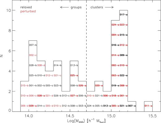
Distribution of M200 for the sample of 62 simulated haloes in our reference (AGN) run. Cluster names correspond to those given in Bonafede et al. (2011), with the addition of D25–D29, which indicate low-mass object re-simulations. The main haloes of each re-simulation are termed DXX–a (bold face), while their satellites are indicated with letters from –b to –e in decreasing mass order. The vertical dashed line indicates the mass limit of 5 × 10¹⁴ h−1 M⊙ used to separate groups (34 objects) and clusters (28). Objects marked in red correspond to perturbed (32) haloes, while black indicates relaxed (30) ones, as defined in Section 3.3.
In order to study the dependence of the clumpiness on the mass of the halo and on its dynamical properties, we divide our objects into subsamples: given the amplitude of our initial sample, this can be done without losing statistical robustness. In particular, we will adopt the following two definitions:
- clusters/groups
(28 and 34 objects, respectively), according to their M200 being higher/lower than 5 × 10¹⁴ h−1 M⊙,
- relaxed/perturbed
(30 and 32 objects, respectively), according to a definition based on the clumpiness, described in Section 3.3.
The histogram of Fig. 1 shows these classifications. It is worthwhile to note that clusters tend to be slightly more perturbed (16 and 12 relaxed) than groups (16 and 18) owing to their more active dynamical state.
DENSITY INHOMOGENEITIES
The gas clumpiness
A commonly used indicator of the degree of inhomogeneity of a medium is its clumpiness. Even though it is normally used to measure the impact of small clumps in an approximately uniform medium, its general definition allows us to use it also to quantify the amount of inhomogeneity associated with large-scale density fluctuations.
For the purpose of our work, for every halo we compute the clumpiness and the other physical quantities in the range 0 < r < 2R200, in 50 equally spaced bins.
Separating small clumps from large-scale inhomogeneities: the residual clumpiness
The amount of clumpiness of the ICM is caused by two phenomena: the presence of small dense clumps, and the density fluctuations on larger scales associated with asymmetries in the large-scale accretion pattern, with the former constituting the dominant contribution. Here we describe a method that is useful for isolating these two components in order to treat them separately. This aspect is particularly important when we consider that the physical properties of clumps and their abundance depend on the processes of cooling and star formation; thus, their presence in our simulated clusters is subject to the uncertainties associated with the implementation of physical models in hydrodynamical codes. Moreover, several works (see e.g. Mitchell et al. 2009; Sijacki et al. 2012, and references therein) have highlighted that SPH simulations produce a higher number of dense clumps than Eulerian ones. This is associated with the different numerical viscosities, intrinsic to the codes themselves, which causes a lower dissipation efficiency in SPH simulations.
We follow the volume-selection scheme described in Roncarelli et al. (2006b) to compute the profiles of galaxy clusters close to and beyond R200. This method consists of sorting the SPH particles belonging to a given radial bin according to their physical density. Then, starting from the most diffuse one, we sum their volumes (defined as Vi = mi/ρi) until we reach a fixed fraction, 99 per cent in our case, of the total volume of the radial bin, and consider only these particles to compute C: the remaining particles are identified as clumps and considered separately in our computation. This procedure proved to be effective in excising all the dense and cold clumps that are highly dependent on the physical assumptions, as well as the small X-ray-bright regions that are usually masked out in observational analyses, thus providing a good description of the global properties of the ICM such as density, temperature and X-ray surface brightness (see the discussion in Roncarelli et al. 2006b). Recently, a similar approach was applied to Eulerian simulations by Zhuravleva et al. (2013), who approximated the density distribution of the gas in different radial bins with a lognormal distribution and marked as clumps the cells with density above values fixed in terms of the σ of the distribution (see also Khedekar et al. 2013). In fact, although applied to completely different numerical schemes (grid-based versus SPH), their method in general corresponds to ours, with their threshold of fcut = 3.5 approximately matching our 99 per cent criterion. Concerning the possible biases caused by unresolved clumpy gas, we have verified that they have a small impact on our results. More details about this point and about the physical properties of clumps are given in Appendix A. We use this method to define the residual clumpiness associated with large-scale perturbations, Cℛ, and to separate it from the total one: this allows us to note that the value of Cℛ is about one order of magnitude lower with respect to C inside R200 (see the discussion in Section 3.3).
We have also checked that in most cases lowering the threshold value to 95 per cent (i.e. increasing by a factor of 5 the volume of gas considered as small-scale clumps) produces negligible changes in Cℛ. However, when the cluster is perturbed by the presence of a large halo (e.g. an infalling group), lowering the density threshold for clump identification can change the final result by up to 50 per cent in the radial bins corresponding to the halo distance. A sketch of the application of this method is shown in Fig. 2 for two cases. These X-ray surface brightness maps show that when cutting the 1 per cent densest volume (from the top to middle panels) we are able to remove all obvious clumpy structures that are associated with the brightest peaks. When cutting 5 per cent of the volume (bottom panels) the surface brightness remains almost unchanged for a relaxed halo (left), while for a dynamically perturbed one (right) the infalling halo on the bottom right is progressively removed, indicating that it is difficult to define a precise threshold to separate the two components. The effect on the definition of Cℛ can be clearly seen in Fig. 3, where we show the residual clumpiness as a function of radius computed for these two haloes by adopting the two volume thresholds: while for D17-a the value of Cℛ is almost independent of the threshold chosen up to R200, for D12-a the presence of the infalling halo at r ≃ 0.5R200 produces a difference of about 0.25.
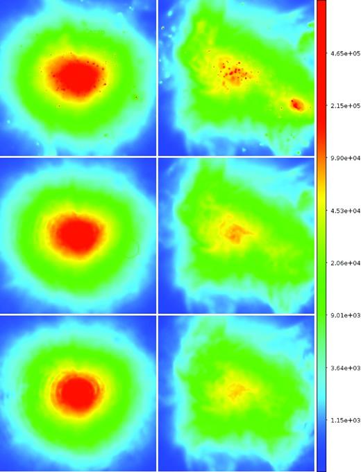
Bolometric (0.1–10 keV) X-ray flux (in units of counts s−1 cm−2) of a relaxed cluster (D17–a, left column) and a perturbed one (D12–a, right column). The size of each map is 1R200 per side. In the first row, all the particles are considered; in the second and third rows, the volume cut has been applied, considering the 99 per cent and 95 per cent thresholds, respectively.
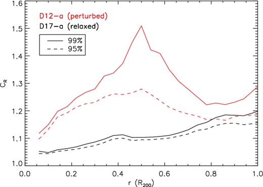
Residual clumpiness as a function of distance from the centre computed for the two haloes shown in the maps of Fig. 2: D17–a (black lines, lower values) and D12–a (red lines, higher values). The value of Cℛ has been computed adopting two different thresholds for the volume-clipping method: 99 per cent (solid lines) and 95 per cent (dashed lines). The physical model assumed is the reference one (AGN).
For this reason we use the difference between the value of Cℛ computed with these two limits to introduce another useful halo classification. We sort our haloes according to the maximum relative difference between C99(r) and C95(r) for r < R200 and split our 62 haloes into two roughly equal subsamples: we define a halo as relaxed when this difference is less than 8 per cent, and as perturbed otherwise. In this way, we end up with 32 perturbed haloes and 30 relaxed ones. For this last set we can consider our value of Cℛ to represent a robust estimate of the degree of inhomogeneity associated with large-scale asymmetries. We also verified that our classification has a good correspondence with an observational-like classification based on X-ray images. We refer the reader to Appendix B for further details on this point.
Dependence on physics and environment
We show in the top panel of Fig. 4 the results of the clumpiness as a function of radius for our whole sample of objects, computed according to the three physical implementations described in Section 2.2. When radiative cooling is included (CSF and AGN models), the level of clumpiness is very high and ranges from ∼3 close to the centre up to ∼10 close to R200. For the outer regions, the value of C increases exponentially, reaching values of the order of 100 at 2R200, with no significant difference when including BH feedback. When neglecting gas cooling (NR), the values drop by a factor of 5–10 over the whole range, indicating that the value of C is associated mainly with small cold clumps.
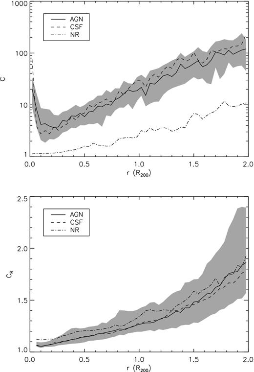
Upper panel: gas clumpiness of our simulated haloes as a function of distance from the centre, for the AGN (solid line), the CSF (dashed) and the NR (dot–dashed) models. The values represent the median of 62 objects; the grey-shaded region encloses the quartiles of the AGN model (the quartile regions of the other two runs have similar sizes). Lower panel: as upper panel, but for the residual clumpiness, that is, after applying our volume-clipping method.
However, when comparing our results with observational estimates it must be noted that the cold dense gas at T < 105 K does not produce any observable clumpiness in X-ray images. This makes the plotted NR profile model a reference for the observed value of C without considering any detection of emitting clumps. For this reason we conclude that the value of ∼16 obtained by Simionescu et al. (2011) for the Perseus cluster is not realistic, as it is sufficient to exclude cold gas from our simulations to obtain significantly lower values.
The lower panel of Fig. 4 shows the values of Cℛ, namely the clumpiness computed after applying the 1 per cent volume-clipping described in Section 3.2. With this method, the difference associated with the physical implementations disappears almost completely, even for the NR model: this indicates that large-scale inhomogeneities do not depend on the physical processes that occur in the ICM, but on the intrinsic dynamical properties of the halo itself. In this case the median of Cℛ computed on the whole sample has a value very close to 1 (i.e. representing an almost uniform medium) close to the centre and increases monotonically up to 1.3–1.4 at R200. There is a significant variance among the haloes, with about 25 per cent of objects having values of ∼1.4. Outside R200 the value of Cℛ reaches ∼2 at 2R200, with an increased dispersion between the objects: this reflects the intrinsic difference between the environments at the outskirts of clusters and groups, which can contain, or not, infalling haloes and accreting filaments.
This independence with respect to the physical implementation is in agreement with what was found by Vazza et al. (2013). However, it is partially in disagreement with what was found by Zhuravleva et al. (2013), who observed a slightly higher degree of inhomogeneity of the bulk in their NR runs, of the order of ΔC = 0.1–0.2. In fact, also in our simulations we see a small (ΔC ∼ 0.04) systematic excess in our NR model, associated with the hot dense tail of the ICM distribution. This discrepancy probably indicates a different cooling efficiency in the simulations analysed here and by Zhuravleva et al. (2013).
It is interesting to see how the trend of Cℛ varies when considering the mass of the halo and its dynamic status. We show in the top panel of Fig. 5 the results of Cℛ computed when separating the haloes according to their mass into groups and clusters (see Section 2.3). Clusters have on average a higher value of Cℛ of the order of ∼0.1, with larger differences outside R200: this is due to the fact that massive objects have a higher probability of accreting material even at later epochs, while galaxy groups are dynamically older, more dynamically stable and, therefore, more uniform. When separating relaxed and perturbed objects according to our definition (see Section 3.2) the difference is even more remarkable, as can be seen in the bottom panel of Fig. 5. While close to the centre the two samples have very similar values of Cℛ, the presence of accreting structures pushes the residual clumpiness of perturbed objects beyond 1.5 at R200. In contrast, relaxed haloes all show the same trend, with Cℛ increasing linearly to 1.3–1.5 at R200: the residual clumpiness of these objects should be considered as an indicator of the degree of inhomogeneity common to all haloes, even the more dynamically stable ones, and connected to their departure from spherical symmetry and to the density fluctuations associated with large-scale accretion patterns.
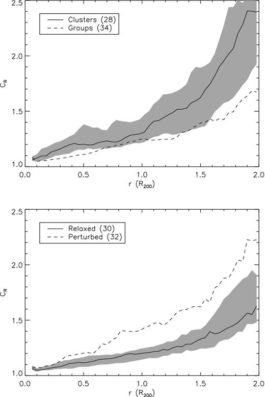
Upper panel: residual gas clumpiness (i.e. after applying the volume-clipping method) for clusters (solid line) and groups (dashed line) as a function of distance from the centre for our reference model. The values represent the median of the sample (28 and 34 objects, respectively), and the grey-shaded region encloses the quartiles of the cluster sample. Lower panel: as upper panel, but with relaxed (30 objects, solid line) and perturbed (32 objects, dashed line) haloes.
We also observe that the differences in Cℛ associated with the cluster/group classification can be explained completely by the different correlation with the relaxed/perturbed classification (i.e. clusters have higher values of Cℛ because they are on average more perturbed than groups), making the latter classification the more interesting for our purposes. We note also that the trends that we observe are similar to those found by Zhuravleva et al. (2013) (we refer to their ‘bulk CSF’ results), both in terms of radial dependence and with respect to the dynamical state of the haloes.
THE AZIMUTHAL SCATTER AS A DIAGNOSTIC OF THE RESIDUAL CLUMPINESS
The azimuthal scatter
As noted, the clumpiness of the ICM is not a directly measurable quantity. Here we investigate the possibility of obtaining an estimate from the observed azimuthal scatter of the X-ray and SZ profiles of the haloes.
We compute the X-ray surface brightness for every halo in the same 50 radial bins and in the 12 sectors by assuming an APEC emission model (Smith et al. 2001), by fixing the redshift of our clusters2 to z = 0. Because our AGN model follows the enrichment of metals with the recipe of Tornatore et al. (2007), we consider also the contribution from various chemical species in the computation of the emissivity of the SPH particles (the details of the procedure are described in Roncarelli et al. 2012). Concerning the SZ scatter, the method to compute the value of the y-parameter from our SPH simulation is the same as in Roncarelli et al. (2007). For these computations we are considering all the SPH particles, without applying the volume-clipping method (see Section 3.2).
We show in the upper panel of Fig. 6 the azimuthal scatter as a function of distance from the centre for the value of the y-parameter and the surface brightness in three X-ray bands. At each distance we show the median computed over the whole sample of 62 haloes in the AGN model. The general observed trend is an increase of the azimuthal scatter with radius, with the value of σy going from ∼0 at the centre to ∼0.3 at R200. The scatter associated with the X-ray surface brightness is 2–3 times higher at all distances, with lower energy bands (0.3–0.8 and 0.5–2 keV) having higher values compared with the hard 2–10 keV band, indicating that these inhomogeneities are associated with gas at temperatures of ∼0.5–1 keV, which has the peak of its emission at soft X-ray energies.
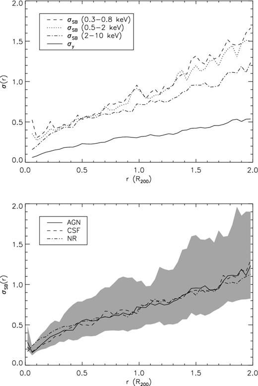
Upper panel: azimuthal scatter of the y-parameter (solid line) and of the X-ray surface brightness in the 0.3–0.8, 0.5–2 and 2–10 keV bands (dashed, dotted and dot–dashed lines, respectively) as a function of distance from the cluster centre. The values represent the median computed over the whole sample of 62 haloes in 12 azimuthal sectors. Lower panel: as upper panel, but for the 2–10 keV surface brightness only, computed with three different physical implementations: AGN (solid line), CSF (dashed) and NR (dot–dashed). The grey-shaded area encloses the quartiles of the cluster sample for our reference model.
It is interesting to note that when studying how the azimuthal scatter varies with respect to the assumed physics and to the halo classifications, its trends are very similar to the Cℛ ones, rather than the ones of the global clumping factor C (refer to Section 3.3). For instance, in the lower panel of Fig. 6 it can be shown that the value of σSB is almost independent of the assumed physical model. When looking at the dependence on the mass and the dynamical status of the halo (upper and lower panels of Fig. 7, respectively) we can see that on average galaxy clusters show a slightly higher azimuthal scatter, while perturbed systems have values of σ that are higher by a factor of 2 with respect to relaxed ones at R200.
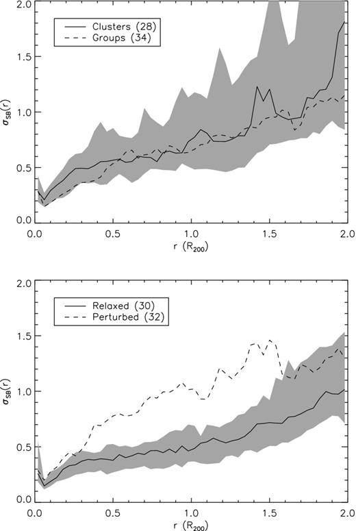
Upper panel: azimuthal scatter of the 2–10 keV surface brightness for clusters (solid line) and groups (dashed) as a function of projected distance from the centre for our reference model. The values represent the median of the two samples (28 and 34 objects, respectively), and the grey-shaded region encloses the quartiles of the cluster sample. Lower panel: as upper panel, but with relaxed (30 objects, solid line) and perturbed (32 objects, dashed line) haloes.
Correlating the clumpiness with the azimuthal scatter
Because we have shown that clumpiness and azimuthal scatter have similar radial trends, here we address directly the question whether a tight correlation exists between these variables and whether there exists a relationship that can connect one with the other.
For this purpose we perform a statistical analysis of these variables by computing the Spearman's rank correlation, rS, of C and of Cℛ with the scatter in the X-ray and SZ profiles of our clusters. We restrict our analysis to the interval 0.15 < r/R200 < 1.5, in order to cut out the core, and to the sample of relaxed haloes, for which the definition of Cℛ is more robust. Given the large sample of haloes available, these restrictions do not affect the robustness of our computation. The results are shown in Table 1.
Spearman's rank correlation (rS) of the values of C and Cℛ (second and third columns, respectively) with the azimuthal scatter in the X-ray surface brightness in various bands (first to third rows, respectively) and in the y-parameter profiles (fourth row). The values analysed are taken from the 30 relaxed haloes considering bins in the range 0.15 < r/R200 < 1.5.
| C | Cℛ | ||
|---|---|---|---|
| σSB (0.3–0.8 keV) | 0.32 | 0.59 | |
| σSB (0.5–2 keV) | 0.30 | 0.60 | |
| σSB (2–10 keV) | 0.23 | 0.61 | |
| σy | 0.35 | 0.68 |
| C | Cℛ | ||
|---|---|---|---|
| σSB (0.3–0.8 keV) | 0.32 | 0.59 | |
| σSB (0.5–2 keV) | 0.30 | 0.60 | |
| σSB (2–10 keV) | 0.23 | 0.61 | |
| σy | 0.35 | 0.68 |
The main conclusion that can be drawn from these results is that the azimuthal scatter of both X-ray and SZ profiles has a very high degree of correlation with the values of Cℛ; that is, with the inhomogeneities on large scales. In fact, the values of rS = 0.6–0.7 indicate that it is possible to describe Cℛ as a monotonic increasing function of σy and σSB. When considering the correlation of the different azimuthal scatters with the total clumpiness, C, however, the correlation is much weaker, although it still exists. It is also worthwhile to point out that the trend with X-ray energy is opposite in the two cases. Because clumps embed lower-temperature ICM, soft bands are more strongly correlated with C than is the hard one. When clumps are excised, however, the densest gas is hotter, and thus the correlation Cℛ–σSB increases at higher energy.
To give more details, we show in Fig. 8 the correlation between Cℛ and the scatter in the 2–10 keV band (top panel): although there is significant dispersion, the trend of increasing clumpiness with increasing values of σSB is clear. The same is true when considering the scatter in the y-parameter (bottom panel). When analysing the dispersion of the relation, the trend of higher values of Cℛ for increasing radii is clear (indicated by the different colours), as already discussed for Figs 4 and 5.
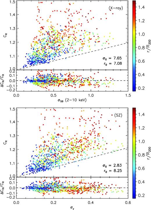
Upper panel: correlation between the azimuthal scatter in the 2–10 keV band and Cℛ. The points considered correspond to the sample of the 30 relaxed haloes in the range 0.15 < r/R200 < 1.5 (a total of 990 points, 33 for each halo), and their colours indicate the radial distance, increasing from blue to red. The quantities indicated (σ0 and r0 in units of R200) are the best-fit values obtained using the formula of equation (6), and the lower part shows the residuals with respect to the model in terms of relative difference in the clumpiness value. The diagonal dashed line indicates the relation Cℛ=1 + σ/σ0, that is, the best-fit formula in the limit of r = 0. Bottom panel: as upper panel, but for the scatter in the y-parameter.
Given the two free parameters, σ0 and r0, for every observable quantity of our analysis (i.e. azimuthal scatter in the X-ray surface brightness and in the y-parameter) we determine their best-fit values by fitting3 the expression of equation (6) using the points displayed in Fig. 8; that is, Cℛ as a function of σ and r. Again, we restrict this calculation to the 30 relaxed clusters and to the range 0.15 < r/R200 < 1.5. The results are shown in Fig. 8, together with the residuals, for the 2–10 keV band and for the y-parameter. It is clear that the best-fit function provides a good global description of the relationship Cℛ–(σ, r), with almost all of the points having an estimate within 10 per cent of the true value. Furthermore, we note how the diagonal dashed line corresponding to the best-fit relationship in the limit of r = 0 defines well the ‘forbidden’ region of the Cℛ–σ plane, below the line itself. Table 2 shows the best-fit values for all three X-ray bands and for the thermal SZ effect.
Best-fit values of the parameters σ0 and r0 (second and third columns, respectively, with r0 in units of R200) of the relation |$C_\rho ^{\rm est}(\sigma ,r)$|, where σ is the azimuthal scatter of the surface brightness in the three X-ray bands (first to third rows) and the scatter of the y-parameter profiles (fourth row). The fourth column shows the median (as a percentage) of the distributions of bias in the value of Mgas at R200 for our sample of 30 relaxed haloes, together with the difference with respect to the upper and lower quartiles (indicated as error), after the clumpiness correction of equation (12). The fifth and sixth columns show the same quantities for the distribution of Mhe and fgas, respectively. In the bottom row we report the values corresponding to the uncorrected biases.
| σ0 | r0 | b(Mgas) per cent | b(Mhe) per cent | b(fgas) per cent | ||
|---|---|---|---|---|---|---|
| σSB (0.3–0.8 keV) | 22.85 | 5.51 | |$+0.02_{- 0.85} ^{+ 1.27}$| | |$-0.56_{- 1.19} ^{+ 1.68}$| | |$+0.26_{- 1.31} ^{+ 2.34}$| | |
| σSB (0.5–2 keV) | 16.02 | 5.87 | |$+0.08_{- 0.94} ^{+ 1.22}$| | |$-0.38_{- 1.19} ^{+ 1.69}$| | |$+0.06_{- 0.98} ^{+ 2.38}$| | |
| σSB (2–10 keV) | 7.65 | 7.08 | |$-0.58_{- 0.67} ^{+ 1.53}$| | |$+0.55_{- 2.63} ^{+ 1.87}$| | |$-0.45_{- 1.34} ^{+ 2.59}$| | |
| σy | 2.83 | 8.25 | |$-0.34_{- 0.89} ^{+ 1.40}$| | |$+0.95_{- 1.47} ^{+ 1.84}$| | |$-1.59_{- 1.27} ^{+ 3.02}$| | |
| No correction | |$+6.11_{- 1.51} ^{+ 1.73}$| | |$-2.22_{- 2.02} ^{+ 1.52}$| | |$+8.45_{- 2.11} ^{+ 2.57}$| |
IMPROVING MASS ESTIMATES
In the previous section we showed that it is possible to obtain an estimate of the large-scale inhomogeneities (Cℛ) from the azimuthal scatter in the X-ray surface brightness and y-parameter. The question that arises is whether it is possible to use the observed value of σ(r) as a function of the distance from the cluster centre to improve the estimates of the gas density profile and, consequently, of the measurement of Mgas and Mhe.
Correcting the gas density profile
As examples, we show in Fig. 9 the application of this method to the two clusters of Fig. 2. The relaxed D17-a cluster (left panel) shows reconstructed density profiles very close to the true value,4 with differences smaller than 2 per cent up to R200. On the other hand, the corresponding uncorrected X-ray profile overestimates the true value by 5–10 per cent over the whole r > 0.4R200 range.
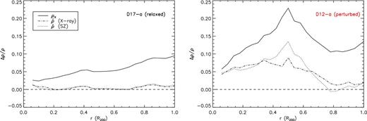
Sketch of the gas density correction method applied to the two clusters shown in the maps of Fig. 2: D17–a (left panel) and D12–a (right panel). We show the radial dependence of the relative differences between the true gas density and the uncorrected measured density (solid line), and the density after applying the X-ray and SZ corrections (dot–dashed and dotted lines, respectively). The horizontal dashed line shows the ideal case of a perfect density profile reconstruction (Δρ = 0).
For the D12-a cluster (right panel), the presence of the disturbing structure still produces an overestimate of the corrected density profiles of about 5–10 per cent at the position of the clumpiness peak. However, even in this case, the improvement with respect to the original ρX profile overestimate is remarkable, through the entire radial range.
This method can be directly applied to the observed density profiles and scatter of Eckert et al. (2012). In fact, these authors obtained a measurement of σSB in the soft 0.5–2 keV band in their 31 ROSAT-PSPC objects (we refer to their fig. 7, the entire sample) up to R200. By using this quantity to estimate the residual clumpiness, we obtain an approximate value of |$C_\mathcal {R}^{\rm est}$| = 1.2 at r ∼R200, which corresponds to an overestimate of ∼8 per cent in the gas density. This consideration mitigates the disagreement between their observed density profiles and the simulated ones, although not by enough to solve the problem completely.
Correcting the gas-mass bias
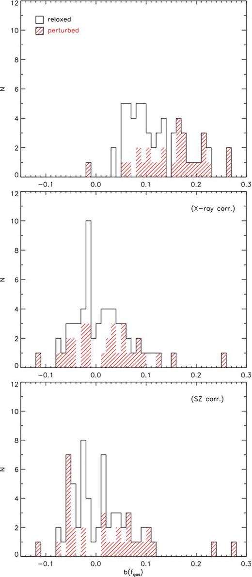
Given our set of simulated clusters and groups, we can obtain the expected value of b(Mgas) from their density and clumpiness profiles. The results are shown in the top panel of Fig. 10: typical values correspond to overestimates of 5–10 per cent, although the more perturbed haloes can reach overestimates of ∼20–30 per cent.
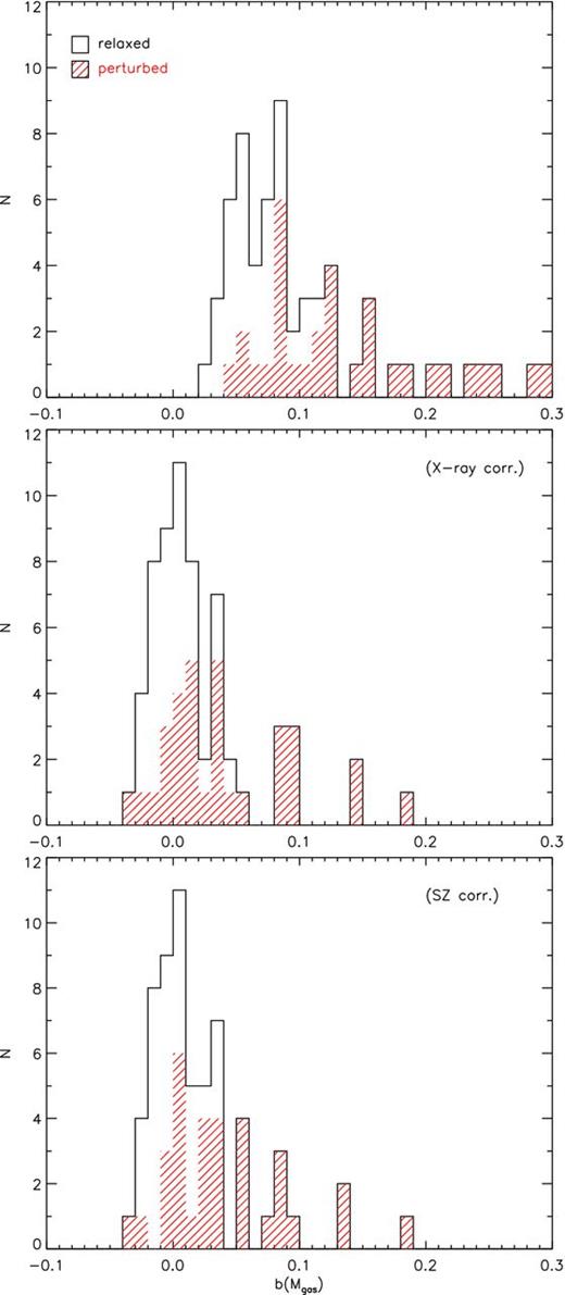
Top panel: histogram of the estimated gas-mass bias associated with the residual clumpiness for our sample of 62 clusters. Perturbed haloes are indicated by the shaded areas. Central and bottom panels: as top panel, but after the correction obtained by estimating the value of Cℛ from the scatter in the 2–10 keV surface brightness and y-parameter, respectively.
We verify the accuracy of this method by applying it to our simulated haloes. The central and bottom panels of Fig. 10 show the distribution of the bias after applying the correction considering the scatter in the 2–10 keV band surface brightness and in the y-parameter, respectively. We also report in Table 2 the values of the median of the corrected and uncorrected bias distributions together with their dispersion for the other two X-ray bands, for our sample of 30 relaxed haloes. In all cases the systematics for relaxed systems is completely eliminated, with the halo-to-halo scatter reduced as well. A very small number of highly perturbed haloes still have overestimates of 10–20 per cent: this reflects the presence of other types of asymmetries in the profiles not directly associated with the clumpiness of the ICM. Nevertheless, when calculating the median and the quartiles of the whole-sample distribution, as shown in Table 3, it can be seen that our method is still effective even if applied ‘blindly’ to all objects.
As Table 2, but for the whole sample of 62 haloes. The best-fit σ0 and r0 are not quoted here, as we assume the same values as for the relaxed sample.
| b(Mgas) per cent | b(Mhe) per cent | b(fgas) per cent | ||
|---|---|---|---|---|
| σSB (0.3–0.8 keV) | |$+1.45_{- 1.54} ^{+ 3.33}$| | |$-0.35_{- 2.58} ^{+ 2.53}$| | |$+2.32_{- 2.86} ^{+ 4.24}$| | |
| σSB (0.5–2 keV) | |$+1.42_{- 1.58} ^{+ 2.99}$| | |$-0.61_{- 2.56} ^{+ 2.60}$| | |$+2.18_{- 2.83} ^{+ 3.85}$| | |
| σSB (2–10 keV) | |$+0.69_{- 1.36} ^{+ 2.76}$| | |$+0.64_{- 3.16} ^{+ 2.80}$| | |$+0.84_{- 3.16} ^{+ 3.56}$| | |
| σy | |$+0.82_{- 1.38} ^{+ 2.72}$| | |$+1.23_{- 2.57} ^{+ 3.17}$| | |$-0.05_{- 3.90} ^{+ 4.80}$| | |
| No correction | |$+8.26_{- 2.54} ^{+ 4.03}$| | |$-2.23_{- 3.59} ^{+ 2.25}$| | |$11.15_{- 3.17} ^{+ 6.16}$| |
In Fig. 11 we show the radial dependence of b(Mgas) and of the corresponding bias after applying the X-ray and SZ corrections. Even close to the core, the uncorrected bias is significant (∼5 per cent) and it grows linearly up to 10 (20) per cent at R200 for relaxed (perturbed) systems. We observe that even at distances corresponding to R500 (≈0.7R200) the expected overestimate is already close to the values at R200, with differences of the order of 2 per cent. When applying the corrections, we can clearly see that for relaxed objects the systematics is completely removed, with a value of 0 ± 2 per cent up to 2R200. Even for perturbed haloes the improvement is consistent (a factor of ∼3) through the whole radial range.
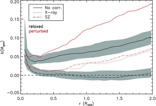
Bias in the value of Mgas as a function of distance from the centre for our reference physical model without correction (solid lines) and with the correction obtained by estimating the value of Cℛ from the scatter in the 2–10 keV surface brightness and the y-parameter (dotted and dot–dashed lines, respectively). The black lines represent the median of the 30 relaxed objects, and the grey-shaded regions enclose the quartiles of the uncorrected and of the X-ray-corrected biases (the quartile region of the SZ-corrected bias has a similar size). The red lines represent the median value for the perturbed sample. The horizontal dashed line corresponds to the value of b(Mgas) = 0.
Correcting the hydrostatic-equilibrium mass bias
The top panel of Fig. 12 shows the distribution of the expected value of b(Mhe) for our sample of simulated clusters and groups. While it is confirmed that for the majority of cases (45 out of 62) the residual clumpiness introduces an underestimate, as the clumping factor of single objects can be affected by local variations [i.e. Cℛ(r) is not perfectly monotonic], the measured Mhe is higher than the true value in about a quarter of our sample. As a general remark, the median effect of about −2 per cent is small when compared with the other systematics, and with respect to the intrinsic dispersion (∼6 per cent difference between the upper and lower quartiles). We note, however, that for the most disturbed systems the error can reach 10 per cent or more in either direction.
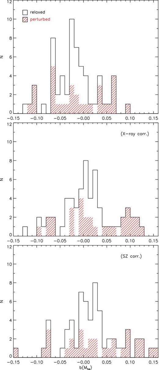
As Fig. 10, but for the bias in the hydrostatic-equilibrium mass. One perturbed halo, D03–a, is not shown because its values are outside the plot range, being, from top to bottom, b(Mhe) = −0.22, −0.21 and −0.19, respectively. D27–a is also outside the plot range in the top and central panels, with b(Mhe) = −0.25 and −0.17, respectively.
We repeat the procedure carried out for b(Mgas) (see Section 5.2) to see whether our clumpiness-correction method is effective in reducing the value of b(Mhe). The results for the three X-ray bands and for the SZ effect are shown in Tables 2 and 3 and in the central and bottom panels of Fig. 12 for the hard 2–10 keV band and for the SZ effect only, respectively. Also in this case we observe a global improvement of the measurements, with the systematics disappearing in all cases. In contrast, the halo-to-halo scatter is not significantly reduced.
Correcting the gas fraction bias
When computing the value of b(fgas) at r = R200 for our sample of 62 haloes, we can see from the distribution shown in the top panel of Fig. 13 that this results in a systematic overestimate of on average about 10 per cent. The ICM inhomogeneities also cause a large spread in the measured value, with 11 objects having b(fgas) > 0.2 (three are outside the plot range).
As Fig. 10, but for the bias in the gas fraction. Three perturbed haloes, D03–a, D18–a and D27–a, are not shown in the top panel as their values are outside the plot range: b(fgas) = 0.35, 0.33 and 0.65, respectively. D27–a is outside the plot range also in the central panel, having b(fgas) = 0.30.
We verify the efficiency of our bias-correction method for fgas by computing the expected value of b(fgas) using the corrected values of b(Mgas) and b(Mhe) (see Section 5.2 and 5.3, respectively) in equation (16). We show the results in Tables 2 and 3 and in the central and bottom panels of Fig. 13 (2–10 keV band and SZ effect only, respectively). Again, in all cases the average bias is significantly reduced, with σSB for the 2–10 keV band and σy providing the best results. In this case, as for b(Mhe), the application of our method reduces the scatter in the measured values.
SUMMARY AND CONCLUSIONS
In this paper we have analysed a set of 62 simulated clusters and groups, obtained with different physical prescriptions, with the objective of providing a global characterization of their density inhomogeneities in the regions close to the virial radius. We have described a method that allows one to separate the ICM clumpiness associated with small clumps from the ‘residual’ one that corresponds to large-scale inhomogeneities, and have discussed how the latter depends on the mass and the dynamical state of the halo. Finally, we have discussed how the presence of large-scale inhomogeneities can bias the estimates of Mgas, Mhe and fgas and have provided a method to reduce this bias by using a directly observable quantity: the azimuthal scatter in the X-ray surface brightness profiles or in the thermal SZ ones (y-parameter profiles).
Our results can be summarized as follows.
As expected, the degree of global clumpiness in our simulated objects depends mainly on the presence/absence of radiative cooling, making about one order of magnitude difference. Once cooling is included, additional feedback mechanisms do not significantly change the clumping factor.
When considering only the contribution of emitting gas, we obtain values of C≃ 2–3 at R200. When compared with the value of ∼16 claimed by Simionescu et al. (2011), we conclude that their estimate cannot be reproduced by our models, even if the whole emitting gas in our simulation is retained.
We introduce the concept of residual clumpiness, Cℛ, to quantify the amount of large-scale inhomogeneities (departure from spherical symmetry, presence of filaments), which can be defined in a robust way for relaxed systems and which corresponds to the bulk clumpiness once obvious bright condensed clumps are masked out. This quantity is independent of the physical model assumed, while it is sensitive to the dynamical state of the halo: relaxed objects have Cℛ∼1.2 at R200, while dynamically perturbed ones have on average Cℛ∼1.5.
The residual clumpiness of the ICM causes a significant overestimate in the measurement of Mgas from X-ray observations, of the order of ∼5–10 per cent for the more relaxed objects and up to ∼20–30 per cent for the more perturbed ones.
A smaller negative bias of about 2 per cent is present also in the measurement of Mhe. Consequently, the combination of the two biases results in an overestimate of fgas, with average values of ∼8.5 per cent, and an intrinsic scatter of ∼9 per cent (interquartile range). These biases are lower than those associated with other systematics.
The residual clumpiness correlates well (rS = 0.6–0.7) with the azimuthal scatter of the X-ray surface brightness and of the y-parameter profiles. This allows us to obtain an analytical formula to estimate it as a function of two observable variables: the azimuthal scatter and the radial distance.
This relationship provides a method to correct the gas density estimates, making it possible to improve consistently the accuracy of the Mgas measurements. With this method, the systematics described above disappears completely for relaxed haloes from outside the cluster core up to 2R200. For perturbed clusters/groups, the overestimate is reduced by a factor of about 3.
Finally, this method also eliminates the bias associated with the measurement of Mhe and fgas. However, a large intrinsic scatter (5–7 per cent, in terms of interquartile range) between the different objects remains.
Overall, our results show how the study of the outskirts of galaxy clusters and groups is important for the measurement of the gas mass and gas fraction, and how the combination of simulations and observations can improve their precision. A possible extension and improvement of this analysis may be obtained by investigating the correlation of Cℛ with other inhomogeneity parameters such as the halo ellipticity, or by determining how the Cℛ(σ, r) relationships may vary as a function of the observed relaxation parameters of the haloes.
Most of the computations necessary for this work were performed at the Italian SuperComputing Resource Allocation (ISCRA) of the Consorzio Interuniversitario del Nord Est per il Calcolo Automatico (CINECA). We acknowledge financial contributions from contracts ASI-INAF I/023/05/0, ASI-INAF I/088/06/0, ASI I/016/07/0 COFIS, ASI Euclid-DUNE I/064/08/0, ASIUni Bologna-Astronomy Dept. Euclid-NIS I/039/10/0, ASI-INAF I/023/12/0, the European Commissions FP7 Marie Curie Initial Training Network CosmoComp (PITN-GA-2009-238356), by the PRIN-MIUR09 ‘Tracing the growth of structures in the Universe’ and by PRIN MIUR 2010-2011 ‘The dark Universe and the cosmic evolution of baryons: from current surveys to Euclid’. DF acknowledges funding from the Centre of Excellence for Space Sciences and Technologies SPACE-SI, an operation partly financed by the European Union, European Regional Development Fund and Republic of Slovenia, Ministry of Education, Science, Culture and Sport. We thank an anonymous referee, who provided useful suggestions for improving the quality of our work. We acknowledge useful discussions with N. Cappelluti, G. Murante, E. Rasia and L. Tornatore. We are grateful to D. Eckert for providing the data on the scatter of his observed profiles.
In this work, R200 is defined as the radius enclosing an average density equal to 200 times the critical density of the Universe, ρc ≡ 3H0/8πG.
Because we are interested in the azimuthal scatter of the X-ray surface brightness and not in its absolute value, fixing the redshift has an effect only in the definition of the X-ray bands.
In the fitting procedure we do not assign errors to our data.
Here we are considering the density profiles after applying the volume-clipping method described in Section 3.2, so we are implicitly assuming that small clumps have been efficiently removed in X-ray observations.
Here we consider only the external part of their profile, namely the formula of their equation (4), after fixing a = 1 and b = 2, thus leaving only three free parameters: normalization, core radius and the external slope c. However, because our objective is to determine the bias associated with the uncertainties in the density profile, any possible effect introduced by changing the temperature fitting procedure is negligible.
REFERENCES
APPENDIX A: IDENTIFYING CLUMPS WITH OBSERVATIONS
Our volume-clipping method, described in Section 3.2 and in more detail in Roncarelli et al. (2006b), allows us to separate the gas belonging to clumps from the bulk of the cluster based on theoretical considerations. Here we provide more information on the physical properties of these clumps and investigate the extent to which they can be detected with simulated X-ray surface brightness maps, and whether the various methods introduce significant biases into the Cℛ determination.
We show in Fig. A1 the T–ρ scatter plot of the SPH particles in the outskirts of the D17-a relaxed cluster, obtained with our reference physical model. The amount of gas that our algorithm associates with the clumpy phase (red and green points) corresponds to about 3 per cent of the total gas mass inside R200 for this halo. We verified that in perturbed systems it is slightly higher (4–5 per cent). When analysing the plot, the multiphase nature of these clumps shows up clearly. Part of the gas is associated with the cold star-forming phase at ρ > 103ρb and T = 104–105 K. These particles are responsible for most of the global ICM clumpiness (see the comments on Fig. 4) but would not influence any X-ray measurement as their temperature is too low to produce any significant emission. The majority of clump particles, which usually embed the previous ones, are instead at a higher temperature (T > 106 K) and can eventually produce a detectable X-ray emission. When neglecting cooling (i.e. the NR run), because the cold dense tail of particles is not present, our method identifies only particles corresponding to the latter phase.
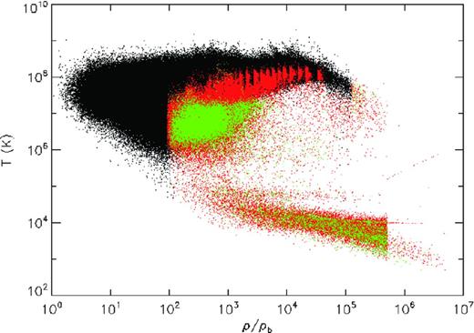
Phase diagram of the SPH particles outside 0.5R200 of the D17–a simulated cluster for our reference model. The black points indicate the particles of the bulk. The particles identified as clumps by our algorithm are marked in green if they fall inside a contour region of the right panel of Fig. A2, and red otherwise.
The maps of Fig. A2 show the 0.5–2 keV surface brightness, up to 2R200 of the bulk (left panel) and of the clumps (right) of the D17-a relaxed cluster, as defined by our method. The high homogeneity of the bulk map shows clearly that no clumpy structure is missed by our filtering method and that any possible detectable inhomogeneities must necessarily be associated with the clump phase. The possibility of detecting them depends on how much brighter their signal is than the bulk one. For this purpose we identified the map regions where the signal-to-noise ratio exceeds a value of 3, by considering the bulk map as a reference for the noise. Most of the clumpy structures are at least partially identified with this method, with an increasing efficiency towards the outskirts.
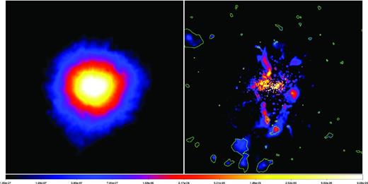
Maps of the soft (0.5–2 keV) X-ray surface brightness of the D17-a cluster for our reference model in units of counts s−1 cm−2 arcmin−2. Each map is centred on the cluster centre and encloses a square of side 4R200. Left panel: the gas identified as ‘bulk’ by our theoretical filtering method (99 per cent volume). Right panel: the gas identified as ‘clumps’ (1 per cent volume). The contours enclose the regions where the projected clumps signal is more than 3 times the bulk one, mimicking a S/N > 3 threshold. As a reference, the typical SPH smoothing length in the outer regions is roughly one-hundredth of the map side.
In Fig. A3 we show the surface brightness of the identified clumps as a function of distance from the centre, compared with the average cluster surface brightness profile. Because the central part of these clumps is usually very bright, in most cases the average surface brightness exceeds the cluster one by more than 5. It is also clear that these structures can be identified outside R200, as their signal is well above the unresolved X-ray background, at least for a massive halo.
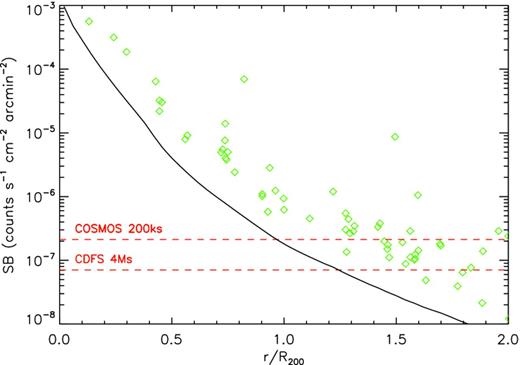
Soft (0.5–2 keV) X-ray surface brightness of the clumps (green diamonds) identified with the method shown in Fig. A2 as a function of distance from the centre. The black solid line represents the average surface brightness of the cluster bulk. The red dashed lines indicate the measurements of the unresolved X-ray background in the same band from the COSMOS survey (Elvis et al. 2009, ∼200 ks exposure, upper line) and from the 4Ms Chandra Deep Field South (Cappelluti et al. 2012, lower line).
As a drawback of our method, we note that in a given radial bin where no clear clumpy structure is present, small fractions of diffuse gas whose signal is not high enough to be identified are considered as clumps. This occurs in particular in regions close to the centre where the ICM is more uniform, as can be seen both in the right panel of Fig. A2 and from the red points of Fig. A2. A precise determination of the fraction of clumps that would be missed by real X-ray observations clearly depends on instrumental details and is beyond the scope of this work, which focuses on large-scale inhomogeneities. However, using our mock maps we can provide an estimate of the amount of missed clumpy gas, together with its influence on the bias of the gas-mass measurements. We verified that the detected clumpy ICM (e.g. green particles in Fig. A2) is ∼20 per cent of the total amount of gas associated with clumps by our volume-clipping method. In order to have an estimate of its impact on the gas-mass measurement, we repeated our analysis by reducing by a factor of 5 the volume threshold (i.e. the 0.2 per cent of the volume of each bin). We obtained a value of b(Mgas) = 7.7 per cent for the relaxed sample, as compared with the previous 6.1 (see Table 2) obtained with our more conservative threshold. Therefore, given the relatively small difference, we conclude that the impact on our results of any unresolved clumpy gas is minor with respect to that associated with large-scale inhomogeneities.
APPENDIX B: RELAXED AND PERTURBED HALOES FROM AN OBSERVATIONAL POINT OF VIEW
In Section 3.2 we described our classification of simulated haloes into relaxed and perturbed according to the robustness of the determination of Cℛ. Here we explain how this criterion, which is based on purely theoretical considerations, actually matches well with a possible classification performed with observational methods.
For this purpose we created a 0.5–2 keV band surface brightness map for each of our simulated objects. Following Cassano et al. (2010), we then computed, over the radial range 0.1–1R200, the centroid shift w, defined as the standard deviation, in units of R200, of the projected separation between the X-ray peak and the centroid, and the power ratio P3/P0 (see Buote & Tsai 1995), which is the lowest normalized moment of the X-ray surface brightness clearly connected to substructures (see e.g. Böhringer et al. 2010). We show in Fig. B1 the position of our simulated systems in the P3/P0 versus w plane. Haloes defined as relaxed according to our definition (marked in black) have on average lower values of all the parameters, thus being located in the lower left corner of the plot, while perturbed ones tend to show a high value for at least one of the two parameters.
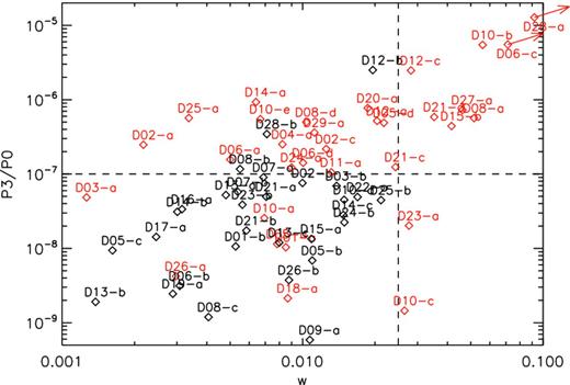
Power-ratio P3/P0 versus the centroid shift w estimated from the 0.5–2 keV surface brightness maps in the radial range 0.1–1 R200 for the sample of our 62 simulated clusters and groups. The two objects indicated with arrows have values outside the plot range. The two dashed lines indicate the limits of w = 0.025 and P3/P0 = 10−7 that provide the best match between the two definitions of relaxed/perturbed haloes (see text).
The dashed lines (w = 0.025 and P3/P0 = 10−7) show the limits that roughly correspond to the best match between the two classifications. When defining observationally the relaxed haloes as the ones found in the bottom-left quadrant of the plot, and as perturbed otherwise, we end up with 53 out of 62 haloes matching the corresponding theoretical definition.
