


Abstract
With the commissioning year of the Large Sky Area Multi-Object Fibre Spectroscopic Telescope (LAMOST), the data archive of one-dimensional spectra is being released gradually. Searching for special objects like cataclysmic variables (CVs) in the data is one of LAMOST's objectives. This paper presents a novel method to identify CVs from optical spectra by using the support-vector machine (SVM) technique combined with principal-component analysis (PCA). After dimension reduction and feature extraction by PCA, spectral data are classified by SVM and most non-CVs are excluded. The final reduced list can be identified manually or by a template-matching algorithm. Experiments show that this data-mining method can find CVs from the LAMOST data base in an effective and efficient manner. We report the identification of 10 cataclysmic variables, of which two are new discoveries. In addition, this method is also applicable to mining other special celestial objects in sky-survey telescope data.
1 INTRODUCTION
The Large Sky Area Multi-Object Fibre Spectroscopic Telescope (LAMOST) is a quasi-meridian reflecting Schmidt telescope with 4000 fibres. The aperture is 4 m, enabling it to obtain spectra of objects as faint as magnitude 20.5. The focal plane is 1.75 m in diameter, corresponding to a 5° field of view (FOV). The light for up to 4000 celestial objects can be directed to the 16 spectrographs simultaneously (Su et al. 1998). The spectral resolution is R = 1000, covering 3700–5900 Å and 5700–9000 Å respectively. It is intended that LAMOST will survey tens of millions of stars, galaxies and quasi-stellar objects (QSOs). It will obtain up to 40 000 spectra per night and the data volume will be several gigabytes. The size of the final data archive will exceed 1 terabyte.
Some test observations have been carried out since the commissioning year of 2009. The pilot survey began in October 2011 and will use half of the available time before the summer shutdown in May 2012. By now, LAMOST has produced over 865 277 spectra in the pilot survey.
Though the core scientific goals of LAMOST focus on extragalactic observations, the structure and evolution of the Galaxy and multiwaveband identification, LAMOST is also ideal for searching for special and faint objects like cataclysmic variable (CV) binary systems.
CVs are close binary stars in which matter is transferred, typically from a low-mass main-sequence star to a white dwarf (WD) via an accretion disc (see Warner 1995; Hellier 2001 for a review). CVs are classified into non-magnetic and magnetic systems based on the strength of the white dwarf's magnetic field. Non-magnetic CVs can be subdivided into dwarf novae and nova-like variables. Magnetic CVs are further subdivided into intermediate polars or polars. Most of the nearly 2000 known or suspected CVs are faint at quiescence and have late-type M dwarf secondaries Downes et al. (2001).1 CVs can emit radiation at all wavelengths from radio and infrared to X- and gamma-rays and are central to our understanding of compact binary evolution, which is central to a variety of astrophysical contexts such as supernovae type Ia, black holes etc. Research on CVs has become more focused in recent years, with more and more CVs discovered. Newfound CVs provide new constraints on binary evolution models (Knigge, Baraffe & Patterson 2011) and contribute greatly to CV orbital period research (Gänsicke et al. 2009; Uemura et al. 2010). Spectroscopic data of CVs can provide a much richer variety of information on both stellar kinematics and stellar atmospheric parameters than is possible with photometric measurements alone. It is necessary to enrich the CV spectral library.
CVs are generally discovered by repeated imaging of the same area of sky, measuring light curves for objects or through photometric surveys. Green et al. (1982) reported 21 CVs from the Palomar Green survey of blue stars. With time-resolved optical spectroscopy and photometry, Aungwerojwit et al. (2005) discovered four long-period CVs in the Hamburg Quasar Survey. A total of 91 CVs were detected during the ROSAT All-Sky Survey (Verbunt et al. 1997). In the Calán–Tololo survey, Tappert, Augusteijn & Maza (2002) detected 12 previously unknown CVs. By cross-matching blue objects from the Sloan Digital Sky Survey (SDSS) with Galaxy Evolution Explorer (GALEX) and the astrometric catalogues USNO-B1.0, GSC2.3 and CMC14, Wils et al. (2010) found 14 new dwarf novae. Szkody et al. (2002, 2003, 2004, 2005, 2006, 2009, 2011)2 used a number of photometric selection criteria to find CV candidates from SDSS, DR1–DR8, and identified 297 new CVs. However, these methods require significant manual processing.
Compared with SDSS, which has its own imaging/photometric survey to select spectroscopic targets, LAMOST does not have its own photometric system and uses a range of available surveys including the Two Micron All-Sky Survey (2MASS: Skrutskie et al. 2006), SDSS (York et al. 2000), United States Naval Observatory B catalog (USNO-B: Monet et al. 2003) and Isaac Newton Telescope Photometric Hα Survey (IPHAS: Drew et al. 2005). LAMOST's photometric information is thus incomplete (Chen et al. 2012; Zhang et al. 2012). It is thus not feasible to use a photometric selection method to find CVs in LAMOST's massive spectra.
The one-dimensional (1D) pipeline of LAMOST is similar to the SDSS SpecBS pipeline (Aihara et al. 2011) and classifies spectra with the method of template-matching (Zhao et al. 2012). At present, LAMOST's 1D pipeline only provides rough classification results and the accuracy is still not robust, especially for some special objects like CVs. Hence, data mining is a practical way to find CVs and will provide a good comparison with LAMOST's 1D pipeline classification.
Astronomical spectral data mining is actually an extension of spectroscopic classification. Stellar spectroscopic classification has been successfully automated by Gulati et al. (1994), Von Hippel et al. (1994) and Singh Harinder, Gulati & Gupta (1998). Their works provide automated stellar classification as well as astrophysical parameters. Current projects using data mining to identify rare objects in massive spectral data sets concentrate mainly on the discovery of supernovae. For example, Madgwick et al. (2003) have detected 19 Ia SNe from 105 galaxy spectra in SDSS-DR1 through the spectroscopic approach. Tu et al. (2009) use the sample reduction and clustering method to find supernova candidates from SDSS DR7.
LAMOST has the advantage of rapidly recording a large number of spectra over a wide solid angle, but has disadvantages such as a bright limiting magnitude and an inability to calibrate spectra accurately. If a real-time data mining system for CVs swas implemented at LAMOST, we could use the shortest possible time to find CVs in more than ten thousand spectra obtained per night and transmit the results immediately to a high-resolution spectrograph like that on the 2.16-m telescope at NAOC (Zhao 2012) for observation in more detail. The two telescopes could be integrated into one more powerful telescope and high-resolution spectra could be achieved at the same time. This system is also well-suited to real-time identification of supernovae, although that is beyond the scope of the current project.
In this preliminary work, we present a new application of a support-vector machine (SVM) combined with principal-component analysis (PCA) to find CVs in LAMOST's spectral data. This is the first attempt to search for CVs in LAMOST's archive and, because there are not enough CV template spectra from LAMOST, we use CV spectra discovered by Szkody et al. (2011) and Patrick et al. (2010) in SDSS as templates to construct the feature space; dimensionality reduction is carried out accordingly. Massive LAMOST spectra are mapped to the feature space and then classified by SVM. Most non-CVs are excluded and the greatly reduced final list of candidates can be identified manually or by template-matching algorithms. Further, the newly identified CVs can be added to the template library, which can make future feature extraction more robust.
This paper is set out as follows. Section 2 describes experimental data, including training data and testing data. In Section 3, we introduce the method used in the paper. In Section 4, we discuss the implementation of the method in detail. In Section 5, we present the results of our experiment. In Section 6, ways to improve the proposed method are discussed. In Section 7, we give our conclusions and outline our plans for future work.
2 THE DATA
The experiment is designed to identity CVs in LAMOST's massive data set by SVM, which depends highly on training data, especially the identified CV spectra. Ideally, training data should be homogeneous with testing data, i.e. LAMOST's raw data. However, LAMOST is still in the pilot phase and there are not enough CV spectra available for training data. It is necessary to find spectra similar to those produced by LAMOST.
SDSS is one of the most ambitious and influential surveys in the history of astronomy (Abazajian et al. 2003). It used a dedicated 2.5-m telescope at Apache Point Observatory, New Mexico, equipped with two powerful special-purpose instruments. The 120-megapixel camera imaged 1.5 deg2 of sky at a time. A pair of spectrographs fed by optical fibres measured spectra of more than 600 galaxies and quasars in a single observation. A custom-designed set of software pipelines kept pace with the enormous data flow from the telescope.
The SDSS spectra have the approximate optical wavelength range of LAMOST and both of the two instruments provide low-resolution, extended wavelength coverage data, as shown in Fig. 1.
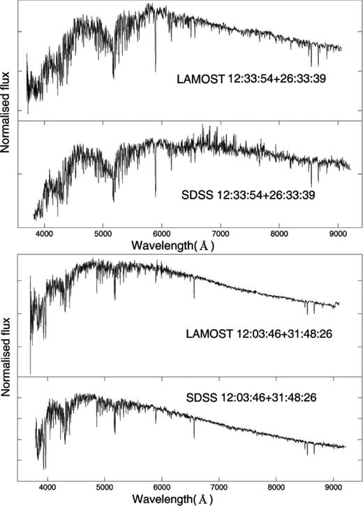
A comparison between LAMOST and SDSS spectra for two stars.
As a result of similar characteristics, the CV spectra discovered by Szkody et al. (2011) and Wils et al. (2010) in SDSS can be used exactly as templates to construct the feature space and for training data after they are preprocessed in the same way (the total number of the spectra is 297 and 12 of them have no spectra or are inaccessible). Most of their discoveries are dwarf novae at quiescence, magnetic CVs and nova-like variables. Thus, it is to be expected that the data-mining results are of similar types. These template spectra are the key to the experiment and four of them are shown in Fig. 2.
CV template spectra from SDSS (the spike near 5575 Å is due to poor subtraction of a strong sky emission line).
The final training data set is the SDSS CV spectra mixed with randomly selected spectra from SDSS including stars, QSOs, galaxies, etc. After pilot survey observations, LAMOST has achieved over 865 277 raw spectral data. This is the experimental data set, i.e. the testing data set in which we perform data mining for CVs. The spectra of LAMOST and SDSS are not exactly identical and should be unified by data preprocessing.
3 METHOD
3.1 PCA
The spectral data of SDSS and LAMOST are high-dimensional. To find CVs in massive amounts of such data, PCA is a popular solution to the problem of dimensionality reduction. Besides, PCA is also employed to construct a subspace (i.e. feature space) in which SVM is used to classify and discriminate between different classifications.
The method of PCA is concerned with explaining the variance–covariance structure of a set of variables through a few linear combinations of these variables. Although all components are required to reproduce the total system variability, often much of this variability can be accounted for by a small number of principal components (PC). There is almost as much information in the partial components as there is in the original variables. The partial principal components are the relatively smaller number of eigenvectors corresponding to the largest eigenvalues; these can replace the initial variables. Each principal component is a linear combination of the original variables. The principal components are orthogonal to each other so that they do not contain redundant information.
The mathematical foundation of PCA is the discrete Karhunen–Loève (K–L) transform. Its purpose is to discover a group of vectors to interpret the variance of data and reduce dimensions by describing the sample with a smaller number of characteristics. More important is the fact that we can construct a feature space afterwards, into which we can map samples for classification (see the review of Shlens 2009).
The method is widely used in astronomical data processing: Qin et al. (2003) used PCA to perform stellar spectra classification; Gaspar (1998) and Zaritsky, Zabludoff & Jeffrey (1995) applied PCA to classify galaxies automatically. McGurk et al. (2010) applied PCA to discuss the correlations of eigencoefficients with metallicity and gravity estimated by the Sloan Extension for Galactic Understanding and Exploration (SEGUE) Stellar Parameters Pipeline.
3.2 SVM
Once the optimal hyperplane is constructed, the classifier is determined and can be used repeatedly, allowing massive data sets to be quickly classified.
SVM has been applied to various astronomical applications such as the selection of active galactic nucleus (AGN) candidates (Yanxia & Yongheng 2003), the determination of photometric redshift (Wadadekar 2005), the classification of galaxies using synthetic galaxy spectra (Tsalmantza et al. 2007) and the morphological classification of galaxies using image data (Huertas et al. 2009). Wozniak et al. (2001) used SVM K means for automated classification of variable stars and compared their effectiveness with that of traditional methods. Humphreys et al. (2001) used decision trees, K–nearest neighbour (Knn) and SVM for classification of the morphological type of galaxy. Their results show that SVM is especially efficient in isolating specific classes from the rest of the observed objects in high-dimensional space.
For the fixed functional form of the kernel, model selection amounts to tuning kernel parameters and the slack penalty coefficient C. The parameter C is the penalty for misclassification, a larger C corresponding to assigning a higher penalty to errors. If C is set large, the number of training errors will be reduced but the classifier performs poorly on testing data (ovefitted). If C is too small, the number of training errors will increase such that the classifier performs poorly on the training set and also may not perform well on the testing data. Generally, one must set C to a fiducial value and check the classification accuracies, then adjust the parameter if needed to obtain a better model.
The performance of SVM is also highly affected by σ: the bigger the σ, the greater the trend of SVM to be a linear classifier; otherwise SVM will be poorly trained or overtrained depending on C.
4 SEARCH FOR CATACLYSMIC VARIABLES
4.1 Data preprocessing
Data preprocessing can often have a significant impact on the performance of the data mining process. If there is much irrelevant and redundant information or noisy and unreliable data, data mining during the training phase will be more difficult. Data preprocessing usually includes data cleaning, rescaling, feature extraction, etc. Kotsiantis, Kanellopoulos & Pintelas (2006) present a well-known algorithm for each step of data preprocessing.
In our experiment, data preprocessing includes low signal-to-noise ratio (SNR) spectra reduction, wavelength unification, raw count rescaling and feature extraction by PCA. The issue of PCA is discussed in a separate section.
The data preprocessing mainly focuses on the following to process the data.
Culling low-SNR spectra. The information contained in LAMOST spectra with SNR < 5 is usually drowned in noise. Most of these spectra are poor quality with various problems and cannot be identified correctly even by manual identification. The 78 898 low-SNR LAMOST spectra are culled in this first step.
Unifying the wavelength to (3800–9000 Å) with fixed step length. The LAMOST spectra cover from 3700–9000 Å and the SDSS spectral wavelength coverage is 3800–9200 Å; therefore the wavelength in our experiment is trimmed to 3800–9000 Å.
- Rescaling the counts with formula (1):where xi is the count of each pixel of the spectrum and M (3522 in our experiment) is the number of pixels per spectrum.(1)\begin{equation} x_i =x_i \Bigg/\sqrt{\sum \limits _{j=1}^M {x_j ^2} }\ , \end{equation}
The final products of LAMOST will be flux-calibrated spectra. At present, the spectra are relatively flux-calibrated with respect to standard star data obtained on the same night in the same spectrograph. Song et al. (2012) proposed a relative flux calibration method by selecting A- and F-type stars as pseudo-standard stars to then estimate their effective temperature and the spectral flux is calibrated by comparing the estimation with stellar models.
However, the present methods are tentative and problematic and can only provide internal units with different scales. The process of rescaling allows LAMOST data and SDSS data on different scales to be compared.
Through the above steps, the data are trimmed to match the wavelength range with accepted S/N and all counts in a spectrum are rescaled to [0, +1].
Additionally, normally one tries to select candidates from photometric information and classify them so that the more expensive procedure of spectroscopy need not be carried out. However, at present there is no strict colour criterion for CVs and the completeness cannot be guaranteed solely with the photometric selection method, even if LAMOST could have complete photometric data like SDSS. Wils et al. (2010) used the photometric selection criteria [(u − g) + 0.85 * (g − r) < 0.18] to search dwarf novae. The colour criterion adopted by Szkody et al. (2002) (u − g < 0.45, g − r < 0.7, r − i > 0.3, i − z > 0.4) applies to WD+M binaries with a few CVs. Their criteria overlap with those of QSOs, faint blue galaxies and white dwarfs. Therefore, photometric selection is not carried out in data preprocessing in our experiment, but if the testing data are similar to SDSS data with photometric information then it is better to use photometric cuts (Yanny et al. 2009) to exclude the doubtless non-CV types first.
4.2 Feature extraction and dimensionality reduction by PCA
The process of PCA is the last step of data preprocessing and is described in detail as follows.
Label SDSS CV template spectra as Pi(i ∈ [1, m]), where m(285) is the number of CV template spectra.
Construct CV template spectra matrix Pm*n, where each row with n (3522) components (the number of pixels per spectrum) is normalized by formula (1).
Construct the correlation matrix of Pm*n: Cn*n = PTn*m*Pm*n.
Calculate and sort in ascending order the eigenvalue of Cn*n.
Once eigenvectors are achieved from Cn*n, order them according to decreasing eigenvalues: λ1, λ2, λ3, … , λn(λi > λj, i > j). The principle components are the eigenvectors corresponding to the largest eigenvalues.
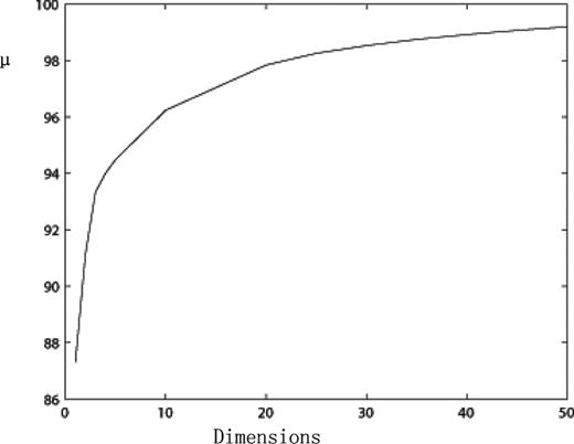
- Use formula (2) to calculate the variance contribution rate μ and construct the transformation matrix E:Results are shown in Table 1 and Fig. 3 respectively.(2)\begin{equation} \mu =\sum \limits _{i=1}^L {\lambda _i } \Bigg/\sum \limits _{i=1}^n {\lambda _i }, \qquad L<n. \end{equation}
The symbol μ represents the proportion of variance of PCA against all variance and the capability of explaining most of the variance in the original data. The parameter μ also controls the final number of dimensions. The higher the μ value, the better the completeness and accuracy of PCA, but the computation will increase sharply accordingly. Thus, maximizing μ with the least number of components is the key to PCA.
In the experiment of Qin et al. (2003), μ reached 98 per cent with the largest two eigenvalues selected. In our experiment we found that μ can reach only 91.13 per cent in the same situation. It can be seen from Table 1 and Fig. 3 that the number of 43 is the point where μ has already reached 99 per cent; it still increases slowly with increasing dimension afterwards. Given the accuracy and computation, the final number of dimensions we choose is 43, which yields a relevant variance contribution rate − μ of 99.01 per cent. To be precise, the top 43 maximal eigenvectors (corresponding eigenvalues λ1, λ2, λ3, … , λ43) are selected and others are abandoned.
Each maximal eigenvector is called an eigenspectrum. The transformation matrix E3522*43 consisting of 43 maximum eigenvectors is the eigenspectra matrix and the corresponding 43-dimensional space is the eigenspace (feature space).
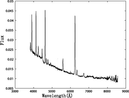
The percentage of the first PC (87.31 per cent) is much larger than that of the other PCs. The first PC is called the max feature spectrum and is plotted in Fig. 4. Obvious He i, He ii and Balmer emission lines can be found in it that are identical to the characteristics of templates. The spike line near 5575 Å is masked and the flux has only mathematical meaning.
Use E3522*43 to project any 3522-dimensional spectra |$\tilde{P}_{1\ast 3522}$| to the 43-dimensional feature space: |$\overline{P} _{1\ast 43}=\tilde{P}_{1\ast 3522}\times E_{3522\ast 43}$|, and a 3522-dimensional spectrum |$\tilde{P}_{1\ast 3522}$| is then transformed to a 43-dimensional spectrum |$\overline{P} _{1\ast 43}$|.
Variance contribution rate.
Variance contribution rate.
| Dimensions | μ (per cent) | Dimensions | μ (per cent) |
|---|---|---|---|
| 1 | 87.31 | 30 | 98.53 |
| 2 | 91.13 | 35 | 98.75 |
| 3 | 93.33 | 40 | 98.92 |
| 4 | 94.00 | 42 | 98.98 |
| 5 | 94.49 | 43 | 99.01 |
| 10 | 96.24 | 44 | 99.04 |
| 20 | 97.84 | 45 | 99.07 |
| 25 | 98.26 | 50 | 99.20 |
| Dimensions | μ (per cent) | Dimensions | μ (per cent) |
|---|---|---|---|
| 1 | 87.31 | 30 | 98.53 |
| 2 | 91.13 | 35 | 98.75 |
| 3 | 93.33 | 40 | 98.92 |
| 4 | 94.00 | 42 | 98.98 |
| 5 | 94.49 | 43 | 99.01 |
| 10 | 96.24 | 44 | 99.04 |
| 20 | 97.84 | 45 | 99.07 |
| 25 | 98.26 | 50 | 99.20 |
Max feature spectrum.
After the above six steps, a 1*3522 spectrum is transformed to a 1*43 spectrum and the sample projection is carried out accordingly. Some information will be lost, but this can be negligible if the eigenvalues are small. With most components left out, the final data will have fewer dimensions and the computation could be significantly reduced.
For visual display of the PCA, in step (5) we set the number of dimensions as three and project samples into a three-dimensional instead of 43-dimensional feature space in Fig. 5. The number of samples is 15 285, namely 15 000 randomly selected LAMOST spectra plus 285 CV templates, all of them are preprocessed in the same way.
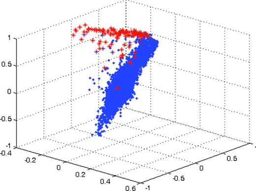
3D projection map (the axes are the first, second and third principle components, respectively).
In Fig. 5, the red and blue asterisks are 285 CV templates and randomly selected LAMOST spectra, respectively. The difference between the two kinds of spectra is obvious in feature space, though a few of them are mixed together. It might be expected that in a higher dimensional space like a 43-dimensional space they can be distinguished completely.
4.3 Sample classification by SVM
The key to sample classification is to train a SVM model and use it to eliminate most of the non-CVs for further manual identification. The model depends highly on a representative training set and parameter optimization.
The training samples consist of two parts. The first part is the 285 identified CV spectra used as positive samples and the second part is the 15 000 randomly selected SDSS spectra used as negative samples.
The negative samples should be composed of most kinds of spectra except CV spectra. The spectral classification of every SDSS spectrum is provided by the SDSS SpecBS pipeline with the keyword SpecClass, according to which we adjust the negative samples to avoid the selection effect of the random selecting algorithm. We also make sure that there are no CV spectra in negative samples through manual review. The distribution of the final negative samples is shown in Table 2.
Distribution of negative samples.
| SpecClass | Proportion (per cent) | Description |
|---|---|---|
| UNKNOWN | 0 | Spectrum not classifiable |
| STAR | 29.48 | Spectrum of a star |
| GALAXY | 24.77 | Spectrum of a galaxy |
| QSO | 36.94 | Spectrum of a quasi-stellar object |
| HIZ_QSO | 1.51 | High-redshift quasar (z > 2.3) |
| SKY | 4.9 | Spectrum of blank sky |
| STAR_LATE | 1.3 | Star dominated by molecular bands M or later |
| GAL_EM | 1.1 | Emission-line galaxy |
Notes: Columns (1) and (3): see Catalog Archive Server (CAS) of SDSS.
Once the training set is determined, transform the data to 43 dimensions with transformation matrix |$\sf{E}$| achieved by PCA. Label CV spectra with label = 1 (positive) and randomly selected spectra with label = −1 (negative). Train the SVM model to get the classifier.
Parameter optimization is a complex subject which is not discussed in detail here; in our experiment we try combinations of C and σ with the range C = [0.001, 0.01, 0.1, 1, 10, 100, 1000] and σ = [0.001, 0.01, 0.1, 0.5, 1, 10, 20] and use grid search with cross-validation to select the best combination. The final accuracy can reach 99.5861 per cent. A visualization of tuning C and σ is shown in Fig. 6.
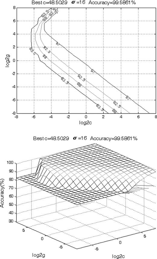
Accuracy contour (top) and surface plot (bottom) of C and σ.
A classifier is achieved with the optimal parameters (C = 48.5029; σ = 16) after the training samples are mapped into the feature space constructed by PCA; then with the classifier we can classify LAMOST spectra quickly. To be precise, the procedure is to transform the testing data, i.e. LAMOST (No. 786, 379) spectra to 43 dimensions with matrix |$\sf{E}$|, label these unknown LAMOST spectra with label = −1, classify the testing data and count the LAMOST spectra with label changed by SVM from label = −1 to label = 1 and denote them as CV candidates.
The LIB-SVM coded by Chih-Jen Lin is adopted in our experiment, which is an implementation of SVM in various kinds of language including Matlab and c.3
5 RESULTS
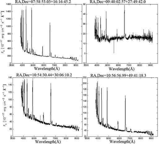
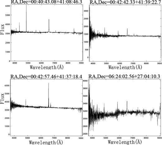
In the experiment, 147 spectra are selected by SVM from LAMOST spectra. 10 of them are identified as definite CVs, of which two are new discoveries. After inspection, we found that 124 of them are poor-quality spectra due to a 2D pipeline and/or low SNR. The other 13 spectra are false positives or by-products, including variable stars, H ii regions or Be stars, i.e. other objects with unusual spectra.
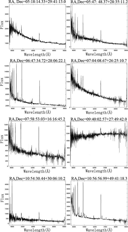
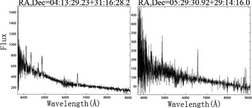
In Table 3, eight known CVs are listed with RA, Dec., GCVS names, subtype, magnitude and references. Their spectra are shown in Fig. 7. In Table 4, the two new discoveries are listed and their spectra are shown in Fig. 8. In Table 5, four objects with unusual spectra are listed; these are shown in Fig. 9.
Known CVs identified by the method. The fluxes of LAMOST spectra are not calibrated and thus are displayed in instrumental units.
Newly identified CVs.
False positives returned by the search.
Known CVs identified by the method.
| RA (J2000) (1) | Dec. (J2000) (2) | GCVS name (3) | Subtype (4) | Mag (5) | Refs (5) |
|---|---|---|---|---|---|
| 05:18:14.33 | 29:41:13.0 | DN | SDSS_i = 15.80 | 1,2 | |
| 05:47:48.37 | 28:35:11.2 | FS Aur | DN | SDSS_g = 16.34 | 3,4,5,6,7,8,9,10,11 |
| SDSS_r = 16.14 | |||||
| SDSS_i = 14.49 | |||||
| 06:47:34.72 | 28:06:22.1 | IR Gem | DN | SDSS_g = 15.98 | 3,4,6,7,9,10,12 |
| SDSS_r = 14.08 | 13,14,15,16 | ||||
| SDSS_i = 16.28 | |||||
| 07:04:08.67 | 26:25:10.7 | V418 Gem | IP | SDSS_g = 16.70 | 17,18,19,20 |
| SDSS_r = 16.91 | |||||
| SDSS_i = 16.92 | |||||
| 07:58:53.03* | 16:16:45.2 | DW Cnc | DN | SDSS_u = 14.80 | 7,10,21,22,23,24 |
| SDSS_g = 15.30 | |||||
| SDSS_r = 14.90 | |||||
| SDSS_i = 15.00 | |||||
| SDSS_z = 15.00 | |||||
| 09:40:02.57* | 27:49:42.0 | DN | SDSS_u = 19.60 | 25,26 | |
| SDSS_g = 19.10 | |||||
| SDSS_r = 18.30 | |||||
| SDSS_i = 17.90 | |||||
| SDSS_z = 17.60 | |||||
| 10:54:30.44* | 30:06:10.2 | SX LMi | DN | SDSS_u = 16.29 | 7,10,25,27,28,29 |
| SDSS_g = 16.74 | 30,31,32,33,34, | ||||
| SDSS_r = 16.46 | |||||
| SDSS_i = 16.39 | |||||
| SDSS_z = 16.43 | |||||
| 10:56:56.99* | 49:41:18.3 | CY UMa | DN | SDSS_u = 17.40 | 5,7,8,9,29,35,36,37 |
| SDSS_g = 17.70 | 38,39,40,41,42,43,44 | ||||
| SDSS_r = 17.50 | |||||
| SDSS_i = 17.30 | |||||
| SDSS_z = 17.10 |
Notes.
Column (1): RA = Right Ascension (J2000); *: also Szkodys CV spectra, see Fig 2.
Column (2): Dec. = Declination (J2000).
Column (3): GCVS = General Catalog of Variables, blank field means no GCVS available.
Column (4): DN – dwarf nova; IP – intermediate polar.
Column (5): Magnitude information of LAMOST derived from catalog of SDSS, 2MASS and USNO etc.
Column (6): References to discovery papers – (1) Witham et al. (2007); (2) Ak et al. (2010); (3) Vogt & Bateson (1982); (4) Williams (1983); (5) Ritter (1990); (6) Bruch et al. (1992); (7) Downes & Shara (1993); (8) Thorstensen et al. (1996); (9) Verbunt et al. (1997); (10) Hoard et al. (2002); (11) Lanning & Meakes (2004); (12) Bond (1978); (13) Szkody, Shafter & Cowley (1984); (14) Ritter (1984); (15) Verbunt (1987); (16) La Dous (1990); (17) Gänsicke et al. (2005); (18) Anzolin et al. (2008); (19) Anzolin et al. (2010); (20) Patterson et al. (2011); (21) Rodriguez Gil et al. (2004); (22) Stepanian (1982); (23) Kopylov et al. (1988); (24) Szkody et al. (2006); (25) Szkody et al. (2007); (26) Krajci & Wils (2010); (27) Sanduleak & Pesch (1984); (28) Wagner et al. (1988); (29) Howell & Szkody (1990); (30) Beasley et al. (1994); (31) Schlegel et al. (1995); (32) Wagner et al. (1998); (33) Ritter & Kolb (1998); (34) Ak et al. (2008); (35) Goranskij (1977); (36) Szkody & Howell (1992); (37) Van Teeseling & Verbunt (1994); (38) Richman (1996); (39) Van Teeseling, Beuermann & Verbunt (1996); (40) Mason et al. (2000); (41) Bicay et al. (2000); (42) Stepanian et al. (2001); (43) Szkody et al. (2005); (44) Witham et al. (2006).
Newly identified CVs.
| RA (J2000) | Dec. (J2000) | Mag |
|---|---|---|
| 04:13:29.23 | 31:16:28.2 | SDSS_g = 17.30 |
| SDSS_r = 16.91 | ||
| SDSS_i = 16.83 | ||
| 05:29:30.92 | 29:14:16 | SDSS_r = 17.18 |
| SDSS_i = 16.82 | ||
| 2MASS_H = 16.81 |
| RA (J2000) | Dec. (J2000) | Mag |
|---|---|---|
| 04:13:29.23 | 31:16:28.2 | SDSS_g = 17.30 |
| SDSS_r = 16.91 | ||
| SDSS_i = 16.83 | ||
| 05:29:30.92 | 29:14:16 | SDSS_r = 17.18 |
| SDSS_i = 16.82 | ||
| 2MASS_H = 16.81 |
False positives returned by the search.
| RA(J2000) | Dec. (J2000) | Type | Mag | Ref |
|---|---|---|---|---|
| 00:40:43.08 | 41:08:46.3 | Infrared source | No | No |
| U_mag = 18.56 | Walterbos & Braun (1992) | |||
| B_mag = 18.73 | ||||
| 00:42:42.33 | 41:39:22.7 | Ionized nebulae in M31 | V_mag = 17.85 | |
| R_mag = 18.22 | ||||
| I_mag = 18.12 | ||||
| U_mag = 18.09 | Vilardell, Ribas & Jordi (2006) | |||
| B_mag = 18.41 | ||||
| 00:42:57.46 | 41:37:18.4 | Variable star | V_mag = 17.77 | |
| R_mag = 17.86 | ||||
| I_mag = 17.66 | ||||
| SDSS_g = 14.99 | No | |||
| 06:24:02.65 | 27:04:10.3 | X-ray source | SDSS_r = 17.60 | |
| SDSS_i = 16.97 |
6 DISCUSSION
The proposed method is implemented on a typical quad-core desktop workstation.
The overall processing time of the experiment is within 8 h and focuses mainly on data reading and preprocessing. Reading data in parallel, like the Message Passing Interface (MPI), should greatly reduce the runtime. Once the PCA transformation matrix |$\sf{E}$| and the SVM classifier are achieved, they can be reused and therefore a new experiment requires less running time. If the number of the experiment data is about 40 000, which is the quantity produced by LAMOST per night, using a high-performance computer the entire processing time should be minutes. Thus the real-time processing requirements can be satisfied.
In general, the SVM training accuracy is used to evaluate the testing accuracy. In this preliminary work, we roughly inspected the testing accuracy by re-identifying the template CV spectra after mixing them with a subset of testing spectra, and the result proved that it is identical with the training accuracy. We would employ other algorithms to inspect objectively and more precisely the performance, completeness and accuracy of the proposed method, including feature extraction, training set selection and parameter tuning.
7 CONCLUSION
We have put forward a data-mining method to search for CVs in massive spectra from the LAMOST data base. The experimental results demonstrate that the method runs efficiently and is able to classify objects in near-real time. Once new CVs of LAMOST are found by the method, they can be reported to other telescopes for follow-up observation. If redshifts of objects can be calculated accurately with the LAMOST 1D pipeline, this method will be especially applicable to supernova searches. We will try it in the next phase of the LAMOST project.
As this is our first attempt at data-mining the LAMOST spectral data, we excluded very low signal-to-noise ratio data. As most of the templates show features of He i, He ii and Balmer emission lines, we do not find galaxies and QSOs in the final results, but rather some emission-line objects with similar spectral features to CVs. As most of them do not show the spectral features of binary systems, these byproducts can be easily distinguished from CVs by eye. This also suggests that the eigenspace constructed by template spectra from the SDSS is not precise enough and needs improvement.
Most of the selected CV template spectra are dwarf novae at quiescence, magnetic CVs and nova-like variables with obvious emission lines. Therefore, the results of our data mining belong to these types. No CV spectrum during outburst is found using the current templates, but expanding the templates to include systems in outburst is feasible.
Because LAMOST is a much more systematic survey, it is expected that with the proposed method it will eventually provide strong constraints on the total number and magnitude distribution of CVs. The LAMOST data archive will be made publicly available in the standard data format for Virtual Observatories and a friendly user interface for this method will be embedded in it, enabling astronomers to explore data interactively.
We are grateful to the anonymous referee for constructive and insightful comments. This paper was proofread by Professor Matt A. Wood. This work is partially supported by the National Natural Science Foundation of China (10973021) and partially by the National Natural Science Foundation of China (11078013). This research has made use of the SIMBAD data base, and also data products from the SDSS and LAMOST.
Information about these sources is available from the online CV catalogue: http://www.astro.washington.edu/users/szkody/cvs/index.html.
SVM is carried out with the existing module developed by Chih-Jen Lin; see http://www.csie.ntu.edu.tw/~cjlin/.
