


Abstract
Angle-dependent partial frequency redistribution (PRD) matrices represent the physical redistribution in the process of light scattering on atoms. For the purpose of numerical simplicity, it is a common practice in astrophysical literature to use the angle-averaged versions of these matrices, in the line transfer computations. The aim of this paper is to study the combined effects of angle-dependent PRD and the quantum interference phenomena arising either between the fine structure (J) states of a two-term atom or between the hyperfine structure (F) states of a two-level atom. We restrict our attention to the case of non-magnetic and collisionless line scattering on atoms. A rapid method of solution based on Neumann series expansion is developed to solve the angle-dependent PRD problem including quantum interference in an atomic system. We discuss the differences that occur in the Stokes profiles when angle-dependent PRD mechanism is taken into account.
1 INTRODUCTION
The solar spectrum shows several lines which are polarized due to scattering of anisotropic radiation on atoms. Such a polarized solar spectrum is called the second solar spectrum (Stenflo & Keller 1996, 1997; Gandorfer 2000, 2002, 2005). It is as structured as the normal intensity spectrum. Some of the strong lines such as Ca ii H&K, Mg ii h&k and the Ca i 4227 serve as probes of the scattering processes taking place in the solar atmosphere. The physics of light scattering on atoms is fully contained in a quantity called partial frequency redistribution (PRD) matrix. It describes the correlations between the frequency, angle and polarization of the incoming and outgoing radiation. The PRD effects are considerably strong in the wings of the lines. For the sake of numerical simplicity, angle-averaged (AA) versions of the PRD functions are often used in line transfer computations. However, a correct treatment of line scattering requires the use of angle-dependent (AD) PRD functions which retain the angle–frequency correlations intact.
The use of AD PRD functions in the line transfer equation dates back to Dumont et al. (1977) and Faurobert (1987), who considered the non-magnetic resonance scattering on atoms. The AD PRD functions in the case of magnetic scattering (Hanle effect) were considered by Nagendra, Frisch & Faurobert (2002) and Nagendra, Frisch & Fluri (2003). These authors solved the transfer problem in the Stokes vector basis. The treatment of AA PRD allows certain level of simplification. Basically, the concerned redistribution matrix (RM) that describes line scattering can be written as a product of a phase matrix (which describes the full polarization and the angular correlations) and the AA redistribution function (which contains the frequency correlations). Such a factorized form for the RM (called hybrid approximation) allowed considerable numerical simplification. Nevertheless, the use of Stokes vector basis kept the inextricable coupling in polarization between the incoming and outgoing rays, making the solution of the concerned transfer problem a time-consuming process. Frisch (2007) introduced an efficient decomposition method based on the expansion of the phase matrix in terms of the so-called irreducible spherical tensors for polarimetry introduced by Landi Degl’Innocenti (1984). This decomposition technique is similar to the earlier methods proposed by Faurobert-Scholl (1991) and Nagendra, Frisch & Faurobert-Scholl (1998) based on the Fourier azimuthal expansion of the phase matrix. However, the decomposition technique of Frisch (2007) is mathematically more elegant and algebraically less tedious. Such a decomposition technique allowed the application of the polarized approximate lambda iteration method to obtain rapid solution of the concerned transfer problem in the irreducible basis (see e.g. Nagendra et al. 1998).
Frisch (2009) presented a decomposition technique for the Hanle scattering problem with AD PRD. This technique makes use of both the irreducible spherical tensor expansion of the Hanle phase matrix and the Fourier azimuthal expansion of the AD PRD function. The corresponding non-magnetic case was discussed in Frisch (2010, hereafter HF10). Recently these powerful techniques were used by Sampoorna, Nagendra & Frisch (2011), Sampoorna (2011), Nagendra & Sampoorna (2011) and Supriya et al. (2012a) to solve different problems of polarized line formation with AD PRD. These techniques, in a modified form (suitable to handle scattering in multi-D media, as well as explicitly AD PRD), are presented in Anusha & Nagendra (2011, 2012). They are subsequently used in Supriya et al. (2012b) to solve the Hanle transfer problem in 1D media.
All the papers mentioned above considered the case of a two-level atom model. In this paper, we extend the above-mentioned techniques to the case of two types of atomic systems. One of them is a two-term atom arising due to fine structure splitting of atomic states, which result in a multiplet. The other atomic system is a two-level atom with hyperfine structure splitting (HFS) of both the upper and lower J-levels taken into account. The scattering in a two-term atom is affected by the interference between the fine structure states – known as J-state interference. The relevant RM that takes into account J-state interference in the upper term was derived by Smitha et al. (2011a, hereafter P1), which is essentially an AD PRD matrix. However, an AA version of this matrix was used by Smitha et al. (2011b, hereafter P2) in line transfer computations in the absence of a magnetic field. The scattering in a two-level atom with HFS is affected by the interference between the F-states. In Smitha et al. (2012, hereafter P3), the relevant RM was derived taking into account the interference between the F-states of the upper J-level, but an AA version of this matrix was used in P3 in the line transfer computations. The purpose of this paper is to solve the transfer problem using AD RM derived for the processes of the J-state interference as well as F-state interference.
In P2, an operator perturbation method was used to solve the transfer problem. In recent years, a faster method of solving the polarized transfer equation is developed based on Neumann series expansion (see Frisch et al. 2009). It is known as scattering expansion method (SEM). Sampoorna et al. (2011), Nagendra & Sampoorna (2011), Sowmya, Nagendra & Sampoorna (2012) and Supriya et al. (2012a) have applied this method to a variety of theoretical problems. In P3, an AA version of the SEM was used to solve the transfer equation. In the present paper, we propose to apply the SEM to solve the radiative transfer equation with AD RM derived for the J-state interference as well as the RM derived for the case of F-state interference.
In Section 2, we present the governing equations of the problem. In Section 3, we present the SEM applied to the problem at hand. Section 4 is devoted to a description of the results. In Section 5, we present the conclusions.
2 GOVERNING EQUATIONS
3 NUMERICAL METHOD OF SOLUTION
4 RESULTS AND DISCUSSION
In this section, we present the emergent Stokes profiles computed using the AD RM for the cases of J-state interference and F-state interference phenomena individually. We consider an isothermal, self-emitting constant property medium characterized by (T, a, ϵ, r, B). T is the optical thickness of the slab and a is the damping parameter. The Planck function is set to unity. The grid used for computations is specified by (Nd, Nx, Nμ, Nφ). Nd denotes the number of depth points per decade in a logarithmically spaced τ-grid with the first depth point at τ1 = 10−2. Nx gives the number of frequency grid points which are very closely and equally spaced in the line cores and in between the lines, and are sparsely but equally spaced in the wings of the lines. Nμ and Nφ specify the number of colatitudes θ(μ) and azimuth angles φ, respectively, for both of which we use Gauss–Legendre quadratures.
4.1 The case of J-state interference with angle-dependent PRD
A two-term atom with an L = 0 → 1 → 0 scattering transition and spin S = 1/2 is considered. The lower and upper terms split into fine-structure levels with J-quantum numbers Ja = Jf = 1/2 and Jb = 1/2, 3/2, respectively. The allowed transition between the J-states gives rise to a doublet at 5000 and 5001 Å. It is assumed that Doppler widths of both these lines are the same and equal to 0.025 Å. The grid used for computation is given by (Nd, Nx, Nμ, Nφ) = (5, 308, 7, 15).
In Fig. 1, we compare the Stokes I profile and the ratio Q/I computed using AA and AD PRD functions including J-state interference effects for different values of optical thickness T. The difference in Q/I obtained using AA and AD PRD is quite sensitive to T and nearly vanish for very thick slabs (like T > 104). For the cases presented in Fig. 1, the AD effects are largest in the PRD wing peaks of 5000 Å line. The antisymmetric PRD peaks about the 5001 Å line and the wavelength region in between the two lines are insensitive to AD effects and are purely controlled by J-state interference effects. In the case of T = 103, the AD effects seem to reduce the asymmetry between the wing PRD peaks of 5000 Å line (brought about by the J-state interference effects), when compared to the corresponding AA case.
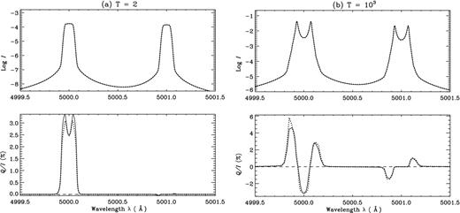
A comparison of emergent Stokes profiles for AD (solid lines) and AA (dotted lines) PRD including J-state interference at μ = 0.0254. A planar slab model with parameters (a, ϵ, r, B) = (10−3, 10−4, 0, 1) are used. Panels (a) and (b) correspond to optical thickness T = 2 and T = 103, respectively.
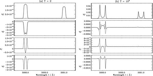
A comparison of emergent |$\mathcal {I}^K_Q$| for AD (solid lines) and AA (dotted lines) PRD including J-state interference at μ = 0.0254. Slab model parameters for the panels (a) and (b) are the same as those of Fig. 1.
4.2 The case of F-state interference with angle-dependent PRD
We consider a two-level atom with J = 1/2 → 3/2 → 1/2 scattering transition and nuclear spin Is = 3/2. Due to HFS, the upper J-state with Jb = 3/2 splits into four F-states with Fb = 0, 1, 2, 3 and the lower J-state with Ja = 1/2 splits into two F-state with Fa = 0, 1. There are six allowed radiative transitions between these F-states which satisfy selection rule ΔF = 0, ±1 and are given in table 1 of P3. Doppler widths of all the lines are again taken to be 0.025 Å. The grid used for the computations is given by (Nd, Nx, Nμ, Nφ) = (5, 417, 7, 15).
In this section, we present the studies analogous to those performed in the case of J-state interference. Therefore, Figs 3 and 4 are analogous to Figs 1 and 2, but for the case of F-state interference. Like in the case of two-term atom with J-state interference and two-level atom with zero nuclear spin, in the present case of F-state interference the difference in Q/I computed with AA and AD PRD are mainly seen in the wing PRD peaks (see Fig. 3) for slabs with T ≤ 103. For slabs with still larger thickness, AD effects are negligible and therefore AA PRD functions can safely be used. Again, these differences can be analysed by studying the irreducible spherical components |$\mathcal {I}^K_Q$| shown in Fig. 4. Further, we have verified that the behaviour of centre to limb variation of I and Q/I profiles for F-state interference case is similar to the corresponding J-state interference case.
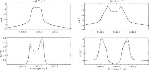
A comparison of emergent Stokes profiles for AD (solid lines) and AA (dotted lines) PRD including F-state interference at μ = 0.0254. A planar slab model with parameters (a, ϵ, r, B) = (2 × 10⁻³, 10−4, 0, 1) are used. Panels (a) and (b) correspond to optical thickness T = 2 and T = 103, respectively.
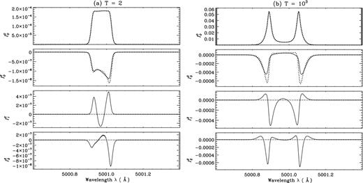
A comparison of emergent |$\mathcal {I}^K_Q$| for AD (solid lines) and AA (dotted lines) PRD including F-state interference at μ = 0.0254. Slab model parameters for the panels (a) and (b) are the same as those of Fig. 3.
5 CONCLUSIONS
We solve the non-magnetic line transfer problem taking into account both the AD PRD and the effects of quantum interference (J-state and F-state interferences individually), and test the validity of using the AA approximation of the PRD (as done in P2; P3) to solve this problem. The studies have been carried out for two types of atomic system (namely a two-term atom with zero nuclear spin and a two-level atom with non-zero nuclear spin) in a collisionless regime and with unpolarized lower level. The decomposition technique developed by HF10 to solve line transfer problem with AD PRD for the case of standard two-level atom with zero nuclear spin is now extended to the case when quantum interference effects are included. This technique helps us to decompose the polarized radiation field into four components that are cylindrically symmetric and satisfy the standard transfer equation. Further, this decomposition technique allows us to solve the transfer equation with AD PRD including quantum interference phenomena using an efficient numerical technique called SEM.
Numerical results for polarized line transfer problem including J-state interference as well as F-state interference are presented. The differences between AA and AD solutions in both the cases are noticed particularly in the near wing PRD peaks. The quantum interference signatures in Q/I are not affected by the AD effects because these effects arise more from atomic physics than from radiative transfer. In both the J-state and F-state interference cases, the differences between AA and AD solutions remain sensitive to the optical thickness T of the slab. The differences are particularly large for slabs of smaller optical thickness (like T ≤ 103), but vanish for very thick slabs. However, over the whole optical depth range the differences never get large enough to be of practical importance for the theoretical modelling of observational data. There is therefore generally no need to invoke the much more computer-intensive AD PRD, since the AA version is accurate enough for all practical purposes.
We thank the referee for a careful reading of the manuscript and constructive suggestions, which helped to improve the quality of the paper.
