


Abstract
We investigate the influence of different thermal and velocity boundary conditions on numerical geodynamo models. We concentrate on the implications for magnetic field morphology, heat transport scaling laws, force balances and generation mechanisms. The field morphology most strongly depends on the local Rossby number, but there is some variation in the dipolarity of the field with boundary condition. Scaling laws also depend on the boundary conditions, but a diffusivity-free scaling is a good first order approximation for all our dipolar models. Our multipolar models, however, obey different scaling laws from dipolar models implying a different force balance in these models. We find that our dipolar models have a stronger degree of Lorentz–Coriolis balance compared to our multipolar models which have a stronger degree of Lorentz-inertial balance.The models with a stronger Lorentz–Coriolis dominance can be generated by either αω, α2ω or α2 mechanisms whereas the models with a stronger Lorentz-inertial balance are all α2 dynamos. These results imply that some caution is necessary when extrapolating results from dynamo models to Earth-like parameters since the choice of boundary conditions can have important effects.
1 INTRODUCTION
Earth's magnetic field is generated in the planet's fluid outer core through dynamo action. In this process, convection and differential rotation of an electrically conducting fluid maintain the magnetic field against its ohmic decay. In the last two decades, 3-D numerical geodynamo models driven by convection in rotating spherical shells have been successful in generating some of the basic properties of the observed geomagnetic field, including the field's dipole dominance, intensity and reversal statistics. This is despite the fact that, due to computational constraints, models operate in a parameter regime that is not representative of planetary interiors (Glatzmaier & Roberts 1996; Kuang & Bloxham 1997; Takahashi et al. 2005; Miyagoshi et al. 2010). A question arises as to how these chosen model parameters, as well as the boundary conditions, affect the numerical solutions. Specifically, since we are interested in determining core properties such as the core–mantle boundary (CMB) heat flux and ohmic dissipation to understand the Earth's heat budget, are dynamo models getting these right? In order to address this question, scaling studies of the influence of model parameters and boundary conditions on dynamo models are required.
1.1 Dynamo scaling laws
As computational capabilities improve, dynamo studies in previously unexplored parameter regimes become feasible. For example, Sakuraba & Roberts (2009) and Miyagoshi et al. (2011) have studied dynamo models at an Ekman number (ratio of viscous to Coriolis force) as low as 10−7. However, the Earth's Ekman number is about 10−15 and hence this example illustrates the many orders of magnitude separating model and planetary parameters. The most practical way to proceed, currently, is to run suites of models using numerically reasonable ranges of parameter values to develop scaling laws between the input and output parameters. The scaling laws must then be assumed to hold over the many orders of magnitude separating model and planetary parameters, and used to infer properties of the geodynamo.
Various studies have developed scaling laws from dynamo simulations for characteristics such as magnetic field strength, heat transport and dipolarity (e.g. Christensen & Tilgner 2004; Aubert 2005; Christensen & Aubert 2006; Olson & Christensen 2006; Takahashi et al. 2008; Aubert et al. 2009; Christensen 2010; Stelzer & Jackson 2013; Yadav et al. 2013). Some important results from these scaling law studies are that (1) the morphology of the magnetic field depends on the local Rossby number (a proxy for the importance of rotation on the convective motions) and (2) diffusivity-free scalings work well for predicting characteristics such as field strength (although a recent analysis calls this into question Stelzer & Jackson 2013). This has lead to the hypothesis that the resulting magnetic field strength depends only on the convective power available to drive the dynamo rather than the balance between Lorentz and Coriolis forces (the so called ‘magnetostrophic balance’ popular in previous literature). The scaling laws developed from these numerical simulations also appear to work well in explaining the field strength for some planets and stars (Christensen et al. 2009).
Most of the models in these simulations use fixed temperature and no-slip boundary conditions although a few of the studies do investigate the effects of some other mechanical and thermal boundary conditions. Several of the studies also incorporate an insulating inner core rather than a conducting inner core, an approximation that can affect force balances in the models (Dharmaraj & Stanley 2012).
1.2 The influence of boundary conditions
Various studies have demonstrated that the choice of thermal and mechanical boundary conditions in numerical models can affect the resulting flows and fields as well as the force balances in the models.
1.2.1 Thermal boundary conditions
Kutzner & Christensen (2000, 2002) studied the magnetic field strength and reversal frequencies of dynamo models for a range of Rayleigh numbers with no-slip velocity boundary conditions and different thermal boundary conditions, with and without internal heating. They found that the choice of thermal boundary conditions made little difference. However, this study utilized a solid inner core that was electrically insulating as opposed to the more physically realistic choice of finitely electrically conducting, and recent work (Dharmaraj & Stanley 2012) has demonstrated that this can affect the results.
Another study on the influence of different thermal boundary conditions showed that at lower Ekman numbers, fixed heat flux models produce Earth-like, strong dipolar magnetic fields, unlike fixed temperature models that produce weak magnetic fields (Sakuraba & Roberts 2009). The difference in the solutions is attributed to large scale circulation, that is strong differential rotation is promoted by fixed heat flux models, which in turn coherently organizes the magnetic field and enhances the dipole component. In the fixed flux models, more heat is transported by convection in the equatorial region than in the polar regions, whereas the fixed temperature models redistribute excess heat more homogeneously at the boundaries.
Hori et al. (2010) studied the influence of thermocompositional boundary conditions on dynamos driven by internal heating. They showed that the impact of the thermal boundary conditions depended on the convective driving source. For example, changing the outer boundary condition only affected the solutions when the driving force was dominated by internal buoyancy sources like secular cooling. Similarly, changing the inner boundary condition only affected the solutions when the dominant driving force was at the inner core boundary, such as the release of light elements or latent heat from a growing inner core. This study was also performed using electrically insulating inner cores, and as mentioned earlier, this may affect the results.
1.2.2 Velocity boundary conditions
Studies provide a variety of results for the influence of different velocity boundary conditions on the dynamo. For example, Kuang & Bloxham (1997) and Kuang (1999) studied the influence of different velocity boundary conditions for a dynamo model with fixed heat flux thermal boundary conditions. They demonstrated that the velocity boundary condition significantly affects force balances in the models. In contrast, Christensen et al. (1999), using fixed temperature boundary conditions, demonstrated that although the choice of velocity boundary conditions influenced the zonal flows that develop in the core, the magnetic field morphology is broadly similar in both cases. Miyagoshi et al. (2010), also using fixed temperature boundaries, demonstrated that at lower Ekman numbers (near the limit of what is numerically achievable currently), the zonal flows are more similar for different mechanical boundary conditions.
Most of the variety in these results is due to the fact that other parameters in these studies are different, for example, different thermal boundary conditions, or control parameter values, or the treatment of the inner core. It would therefore be advantageous for a single study to systematical vary all the boundary conditions to determine the implications.
1.3 Dynamo generation mechanisms
Dynamo models have also been used to investigate the magnetic field generation mechanism in Earth's core (Christensen & Olson 1998; Christensen et al. 1999; Kuang 1999; Olson et al. 1999). The process by which differential rotation can produce toroidal magnetic field is known as the ‘ω effect’. The process by which helical convective upwelling produces both toroidal and poloidal magnetic fields is known as the ‘α effect’. If the toroidal magnetic field is dominantly produced by the ω effect then the dynamo is known as the ‘αω dynamo’, if it is dominantly produced by α effect then the dynamo is known as the ‘α2 dynamo’ and if α and ω effects are equally important, the dynamo is known as the ‘α2ω dynamo’. For a schematic illustration of the generation of poloidal from toroidal magnetic field and vice versa we refer the reader to Olson et al. (1999).
The generation mechanism of the dynamo depends on the force balance. Non-magnetic convection models demonstrate that the flow in a rapidly rotating spherical shell is organized by the Coriolis force into axial columns and the main force balance is between the Coriolis force and the pressure gradient force. In a dynamo model, the addition of a strong magnetic field can influence the fluid motion, breaking the axial column and the competition between the Coriolis, viscous and inertial forces has to accommodate the Lorentz force. It is often assumed that the influence of magnetic field will be important when the Elsasser number (ratio of Lorentz to Coriolis force) > O(1). However, recent studies have shown that the traditional definition of the Elsasser number is not a good representation of the Lorentz to Coriolis force balance. Dharmaraj & Stanley (2012) demonstrated that a comparison of the axisymmetric ϕ component of the Lorentz and Coriolis forces gives a better estimate of the Lorentz–Coriolis balance whereas Soderlund et al. (2012) showed that calculating volume integrals of the forces can do so as well.
In this paper, we use numerical dynamo models to investigate the influence of different thermal and velocity boundary conditions on scaling laws and dynamo generation mechanisms. In Section 2, we describe our numerical model and in Section 3 we present our results. The conclusions are then given in Section 4.
2 NUMERICAL MODEL
The control parameters, boundary conditions and results are summarized in Table S1 for dynamo models and Table S2 for pure thermal convection models with no magnetic field. The boundary conditions given in the supporting tables are applied at both the inner and outer core boundaries. In all the dynamo models presented in this paper, the inner and outer cores have the same electrical conductivities. In our models, the inner core is free to oscillate in response to magnetic and viscous torques. Since we compare models with different thermal and velocity boundary conditions, for convenience, we will use the abbreviations: FFSF for fixed heat flux and stress-free models, FFNS for fixed heat flux and no-slip models, FTSF for fixed temperature and stress-free models and FTNS for fixed temperature and no-slip models. To differentiate between dynamo models and pure thermal convection models with no magnetic field, we use a suffix ‘C’ for ‘convection’ in the boundary condition abbreviation mentioned above. The simulations were run for many magnetic dipole diffusion times and the results presented were analysed after the initial transients decayed.
3 RESULTS
3.1 Dynamo regimes and scaling laws
3.1.1 Dynamo regimes
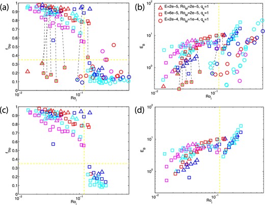
Relative dipole strength and magnetic energy versus local Rossby number: (a) relative dipole strength versus local Rossby number, and (b) magnetic energy versus local Rossby number. The bistable models are connected with a black dashed line. Panels (c) and (d) are (a) and (b) with the bistable models removed, Nu > 2 and E < 6.5 × 10⁻⁵. Red denotes fixed flux and stress-free (FFSF) models, magenta denotes fixed flux and no-slip (FFNS) models, blue denotes fixed temperature and stress-free (FTSF) models, cyan denotes fixed temperature and no-slip (FTNS) models, and a green plus sign inside the symbols denotes bistable models.
For a given Rol in the dipolar regime, the dipolarity fdip does weakly depend on the boundary conditions. As can be observed in Fig. 1, fixed temperature models are generally more dipolar than fixed flux models. For the fixed flux models, stress-free models are more dipolar than no-slip models (ignoring the weak bistable solutions).
3.1.2 Heat transport
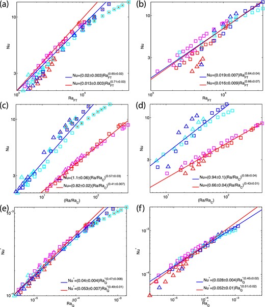
Heat transfer power laws: dynamo models are shown in the left-hand column and convection models with no magnetic field are shown in the right-hand column. The first row plots Nusselt number versus Rayleigh number. The second row plots Nusselt number versus Rayleigh number normalized by it's critical value. The third row plots the modified Nusselt number versus modified flux based Rayleigh number. Symbols as in Fig. 1 without the non-dipolar bistable models. The brown plus signs inside symbols denote multipolar models which have not been included when determining the best-fitting lines since they appear to diverge from the trend. The blue and red lines denote power law fits for fixed temperature (blue and cyan symbols) and fixed heat flux (red and magenta symbols) models, respectively.
The effect of different boundary conditions can be seen more clearly by plotting Nu versus the supercriticality (Ra/RaC) rather than versus Ra. In Figs 2(c) and (d), we see a clear difference between the fixed flux and fixed temperature models, even though there is a significant amount of scatter, especially in the fixed temperature models. Also, the power-law exponents (i.e. the line slope) of all the dipolar dynamo models are similar to the non-magnetic convection models, and the dipolar dynamo models obey similar scaling laws irrespective of the velocity boundary conditions.
3.2 Field morphology
In order to understand the influence of different boundary conditions on the models, we select specific ‘characteristic’ models with the following identical parameters: E = 6 × 10⁻⁵, RoM = 2 × 10− 5 and qk=1 but varying boundary conditions and dipolarity. Since the Rayleigh number is defined differently for fixed flux and fixed temperature models, we choose our characteristic models at similar Nusselt numbers. The characteristic dipolar dynamo models at Nu ≈ 5 are: FFSF-21, FFNS-15, FTSF-15 and FTNS-24, and the characteristic multipolar dynamo models at Nu ≈ 11.5 are: FTSF-20 and FTNS-33. The corresponding non-magnetic convection models at similar Nusselt number are: FFSFC-16, FFNSC-14, FTSFC-09, FTNSC-08, FTSFC-13 and FTNSC-15. The control parameters and boundary conditions of the models are given in Table 1.
Characteristic model results. The column headings are: model ID, Rayleigh number (Ra), supercriticality of Rayleigh number (|$\frac{{\rm Ra}}{{\rm Ra}_C}$|), magnetic energy (EB), kinetic energy (Ek), ratio of poloidal to toroidal magnetic energy (|$\frac{E_{B_P}}{E_{B_T}}$|), relative dipole strength (fDip), Rossby number (Ro), local Rossby number (Rol), Nusselt number (Nu), Match Coefficient of the Lorentz to Coriolis force (MLC) and the Match Coefficient of α and ω effects (Mα and Mω), respectively. All models use hyperdiffusivity parameter l0 = 30. All models were run for at least three magnetic dipole diffusion times and results are based on analysis after the system equilibrated.
| Dynamo models: E = 6.00e–05 , RoM = 2.00e–05, qk = 1, |$N_{r_0}=64$| | ||||||||||||
|---|---|---|---|---|---|---|---|---|---|---|---|---|
| Model | Ra | |$\frac{{\rm Ra}}{{\rm Ra}_C}$| | EB | Ek | |$\frac{E_{B_P}}{E_{B_T}}$| | fDip | Ro | Rol | Nu | MLC | Mα | Mω |
| FFSF-21 | 2.50e+04 | 87.41 | 8.1e+00 | 3.2e+05 | 8.8e−01 | 8.3e–01 | 1.1e–02 | 4.6e–02 | 5.36 | 0.45 | 0.39 | 0.23 |
| FFNS-15 | 2.00e+04 | 82.99 | 4.5e+00 | 1.6e+05 | 1.0e+00 | 7.5e–01 | 8.1e–03 | 3.0e–02 | 5.21 | 0.42 | 0.52 | 0.17 |
| FTSF-15 | 5.00e+03 | 14.49 | 4.6e+00 | 3.1e+05 | 1.3e+00 | 9.3e–01 | 1.1e–02 | 5.5e–02 | 5.06 | 0.36 | 0.41 | 0.27 |
| FTNS-24 | 5.00e+03 | 18.05 | 6.6e+00 | 1.7e+05 | 1.3e+00 | 8.1e–01 | 8.3e–03 | 3.4e–02 | 5.05 | 0.47 | 0.39 | 0.32 |
| FTSF-20 | 2.00e+04 | 57.97 | 1.2e+01 | 4.8e+06 | 8.1e-01 | 1.7e–01 | 4.4e–02 | 1.5e–01 | 11.74 | 0.09 | 0.60 | 0.19 |
| FTNS-33 | 3.00e+04 | 108.30 | 1.3e+01 | 3.3e+06 | 9.1e−01 | 9.7e–02 | 3.6e–02 | 1.4e–01 | 11.75 | 0.02 | 0.67 | 0.12 |
| Convection models: E = 6.00e–05 , RoM = 2.00e–05, qk = 1, |$N_{r_0}=64$| | ||||||||||||
| Model | Ra | |$\frac{{\rm Ra}}{{\rm Ra}_C}$| | Ek | Ro | Rol | Nu | ||||||
| FFSFC-16 | 3.50e+04 | 122.38 | 1.5e+07 | 7.6e–02 | 8.6e–02 | 4.83 | ||||||
| FFNSC-14 | 2.50e+04 | 103.73 | 5.9e+05 | 1.5e–02 | 3.7e–02 | 5.20 | ||||||
| FTSFC-09 | 7.50e+03 | 21.74 | 6.5e+06 | 5.1e–02 | 5.4e–02 | 4.87 | ||||||
| FTNSC-08 | 5.00e+03 | 18.05 | 4.2e+05 | 1.3e–02 | 4.1e–02 | 4.65 | ||||||
| FFSFC-13 | 2.00e+04 | 69.93 | 2.6e+06 | 3.2e–02 | 4.3e–02 | 3.96 | ||||||
| FTNSC-15 | 3.00e+04 | 108.30 | 1.0e+07 | 6.3e–02 | 1.8e–01 | 11.63 | ||||||
Scaling laws for dynamo and non-magnetic convection models. The subscript C denotes convection models. ▵a and ▵b are standard errors in the offset or Y-intercept (a) and slope (b), respectively. These power laws are obtained for models with Nu > 2 and E < 3 × 10⁻⁴. Dipolar dynamo models have fDip > 0.35 and multipolar dynamo models have fDip < 0.35. Ignore the polarity for convection models.
| a ± ▵a | b ± ▵b | aC ± ▵aC | bC ± ▵bC | |
|---|---|---|---|---|
| |${\rm Nu} = (a \pm \triangle a) \ {\rm Ra}_{FT}^{(b \pm \triangle b)}$| | ||||
| All | 0.034 ± 0.004 | 0.59 ± 0.01 | 0.017 ± 0.005 | 0.65 ± 0.03 |
| Dipolar fixed temperature | 0.02 ± 0.003 | 0.65 ± 0.02 | 0.019 ± 0.007 | 0.64 ± 0.04 |
| Dipolar fixed flux | 0.013 ± 0.003 | 0.71 ± 0.03 | 0.016 ± 0.009 | 0.66 ± 0.07 |
| Multipolar fixed temperature | 0.38 ± 0.1 | 0.34 ± 0.03 | ||
| |${\rm Nu} = (a \pm \triangle a) \ (\frac{{\rm Ra}}{{\rm Ra}_C})^{(b \pm \triangle b)}$| | ||||
| All | 1.6 ± 0.2 | 0.33 ± 0.03 | 1.6 ± 0.4 | 0.3 ± 0.06 |
| Dipolar fixed temperature | 1.1 ± 0.06 | 0.57 ± 0.03 | 0.94 ± 0.1 | 0.58 ± 0.04 |
| Dipolar fixed flux | 0.82 ± 0.02 | 0.41 ± 0.007 | 0.66 ± 0.04 | 0.43 ± 0.01 |
| Multipolar fixed temperature | 3.7 ± 0.5 | 0.25 ± 0.03 | ||
| |${\rm Nu}^* = (a \pm \triangle a) \ {\rm Ra}_Q^{*(b \pm \triangle b)}$| | ||||
| All | 0.027 ± 0.002 | 0.43 ± 0.007 | 0.033 ± 0.004 | 0.47 ± 0.01 |
| Dipolar fixed temperature | 0.04 ± 0.004 | 0.47 ± 0.008 | 0.028 ± 0.004 | 0.45 ± 0.02 |
| Dipolar fixed flux | 0.053 ± 0.007 | 0.49 ± 0.01 | 0.052 ± 0.01 | 0.51 ± 0.02 |
| Multipolar fixed temperature | 0.0074 ± 0.001 | 0.28 ± 0.02 | ||
3.2.1 Surface magnetic field
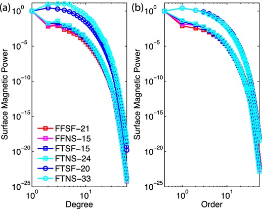
Surface magnetic power spectra: Left-hand plot shows power versus degree normalized to the dipole (l=1) power and the right-hand plot shows power versus order normalized to axisymmetric (m = 0) power. The m = 0 power in the right-hand figure is artificially plotted at m = 0.4 in order to use a log axis.
3.2.2 Magnetic field
In this section, we examine the characteristics of the dynamo models inside the dynamo generation region to understand the difference in the potential fields observed outside as described in the previous section. The magnetic energies of the characteristic multipolar models (that are found at higher Rol) are approximately twice as strong as their respective characteristic dipolar models with similar boundary conditions. The toroidal magnetic field intensities are approximately equal in magnitude to the poloidal magnetic field intensity in all the characteristic dipolar and multipolar models. The multipolar dynamo models are dominated by their non-axisymmetric toroidal and poloidal magnetic fields, whereas the dipolar dynamo models have approximately equal contribution from their axisymmetric and non-axisymmetric components.
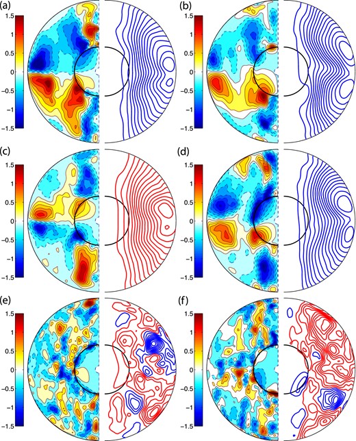
Next we examine the magnetic field morphology of dipolar and multipolar dynamos with different boundary conditions at the CMB and inside the dynamo generation region. Although Figs 4 and 5 present snapshots in time of the resulting magnetic fields of the characteristic dipolar and multipolar models, their features are similar at other times. Fig. 4 presents the radial magnetic field at the CMB. In the dipolar regime, all the models produce strong magnetic field that is mainly dipolar with some non-axisymmetric features, whereas the models in the multipolar regime produce intense small-scale non-dipolar and non-axisymmetric magnetic fields at the CMB as expected. Even though the fixed flux models produce dipolar dynamos, they produce intense patches at the poles, whereas the fixed temperature models are more homogeneous.
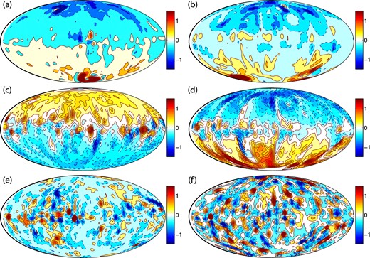
Radial magnetic field at the core mantle boundary: for (a) FFSF-21, (b) FFNS-15, (c) FTSF-15, (d) FTNS-24, (e) FTSF-20 and (f) FTNS-33 models. Red and blue colours represent different field directions. The units are non-dimensional.
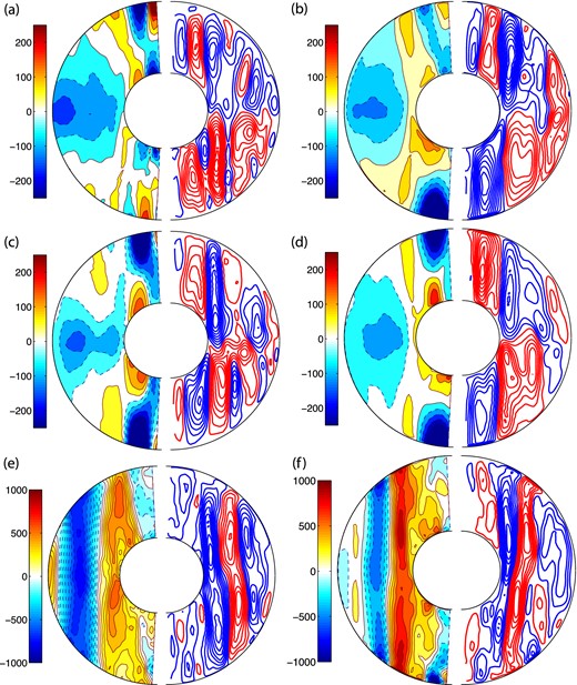
Axisymmetric magnetic field: for (a) FFSF-21, (b) FFNS-15, (c) FTSF-15, (d) FTNS-24, (e) FTSF-20 and (f) FTNS-33 models. The left-hand (right) plot shows the meridional slice of the axisymmetric toroidal (streamlines of poloidal) magnetic field. In the toroidal plots, red shades represent prograde direction and blue shades represent retrograde direction. In the poloidal plots, red is clockwise and blue is anticlockwise. The units are non-dimensional.
Fig. 5 presents axisymmetric meridional slices of the toroidal and poloidal magnetic fields. The magnetic field morphologies of the models in the dipolar regime are different from the models in the multipolar regime. The dipolar models produce large scale toroidal flux patches that are antisymmetric at the equator while the multipolar models produce small scale flux patches that are scattered in the bulk of the outer core. The magnetic field morphology does not strongly depend on the choice of thermal or velocity boundary conditions.
3.2.3 Velocity field
In this section, we examine the characteristics of the flow velocities inside the dynamo generation region and compare them to non-magnetic convection models at similar parameters and boundary conditions. The kinetic energies of the characteristic multipolar dynamo models are an order of magnitude bigger than the dipolar dynamo models. All the characteristic dynamo models are dominated by their toroidal kinetic energies, but the dominance is more prominent in the stress-free models. The characteristic dipolar dynamo models are dominated by the non-axisymmetric component of the toroidal kinetic energies, whereas the characteristic multipolar dynamo models have equal contribution from the axisymmetric and non-axisymmetric components.
The kinetic energies of the characteristic non-magnetic convection models are an order of magnitude bigger than their corresponding characteristic dynamo models. All the characteristic non-magnetic convection models are also dominated by their toroidal kinetic energies. Again, the dominance is more prominent in the stress-free models. Unlike the dynamo models, the toroidal energy is dominated by its axisymmetric component for all non-magnetic convection models.
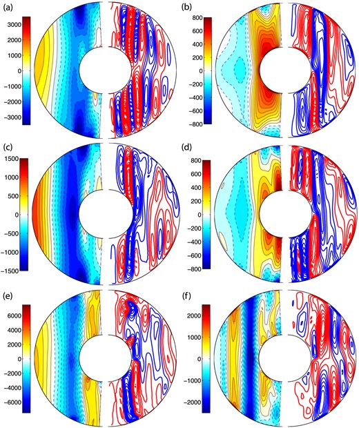
Next, we examine the velocity field morphology of characteristic dynamo models and compare them to non-magnetic convection models. Figs 6 and 7 present typical snapshots of the axisymmetric velocity fields for dynamo models and non-magnetic convection models, respectively. The velocity fields of the models in the dipolar regime are different from both the models in the multipolar regime and the convection models with no magnetic fields. The zonal flows of the multipolar models are stronger than the dipolar models. The toroidal velocity fields of the convection models with no magnetic field are approximately constant on cylinders parallel to the rotation axis, a sign of strong Taylor–Proudman influence. The velocity field morphologies of the multipolar models are similar to the convection models (also seen by Aubert 2005) even though they produce strong magnetic fields. In this case, the strong magnetic fields of multipolar models do not influence the large scale velocity fields.
Axisymmetric velocity field: for (a) FFSF-21, (b) FFNS-15, (c) FTSF-15, (d) FTNS-24, (e) FTSF-20 and (f) FTNS-33 dynamo models. The toroidal velocity fields are shown on the left-hand side where red (blue) denotes prograde (retrograde) circulation and streamlines of poloidal velocity fields are shown on the right-hand side where red (blue) denotes clockwise (anticlockwise) circulation.
Axisymmetric velocity field: for (a) FFSFC-16, (b) FFNSC-14, (c) FTSFC-09, (d) FTNSC-08, (e) FTSFC-13 and (f) FTNSC-15 convection models with no magnetic field. The toroidal velocity fields are shown on the left-hand side where red (blue) denotes prograde (retrograde) circulation and streamlines of poloidal velocity fields are shown on the right-hand side where red (blue) denotes clockwise (anticlockwise) circulation.
On the other hand, the dipolar models have strong differential rotation inside the tangent cylinder and a retrograde equatorial jet outside the tangent cylinder close to the outer core boundary; a sign that Lorentz forces are strong enough to break the Taylor–Proudman constraint. The meridional circulation of the dipolar dynamo models are predominantly equatorially antisymmetric throughout the core. The intensity of the zonal flows of the dynamo models are weaker than the convection models without magnetic field due to magnetic braking. Notably, the velocity field morphologies do not strongly depend on the choice of thermal or velocity boundary conditions.
3.3 Force balances
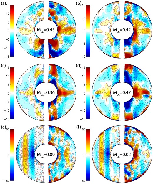
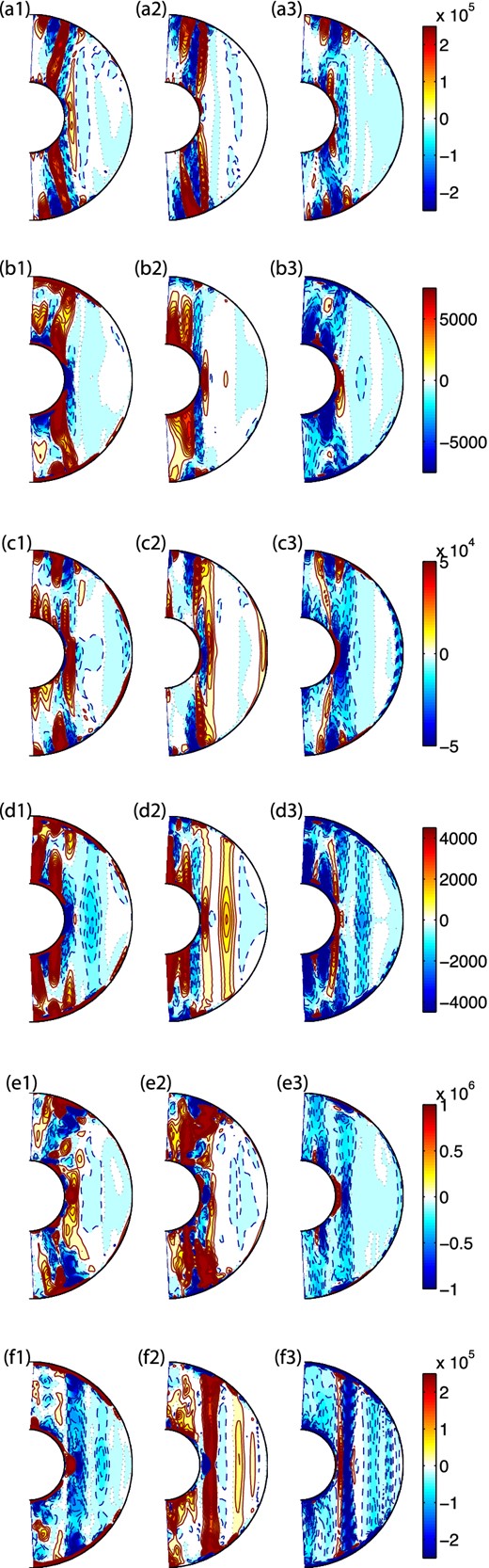
Force balance: for (a) FFSF-21, (b) FFNS-15, (c) FTSF-15, (d) FTNS-24, (e) FTSF-20 and (f) FTNS-33 models. The left- and right-hand plots show the time averaged axisymmetric ϕ components of the Lorentz and Coriolis forces, respectively. The Match Coefficient for the Lorentz and Coriolis forces is also given. For comparison, the more standard measure of normalized correlation coefficients (eq. 26) for the models are (a) 0.7, (b) 0.52, (c) 0.72, (d) 0.44, (e) 0.15 and (f) −0.09. Note that the reported values are calculated by computing the instantaneous match coefficients and correlations and then averaging those values over time.
We also report these values in the Fig. 8 caption. We prefer the Match Coefficient defined in eq. (25) since it computes point-by-point normalization rather than an overall normalization.
As seen in Fig. 8, the models in the dipolar regime have a much higher degree of magnetostrophic balance than the models in the multipolar regime. This figure only shows the degree of correlation of the ϕ-averaged forces, that is those that accelerate a zonal flow, whereas our Match Coefficient measures a more detailed balance including the non-axisymmetric components. Since the multipolar models are dominated by their non-axisymmetric components we examined the force balance due only to the non-axisymmetric components (not shown here) and found that they were also not in magnetostrophic balance. It is evident that the strong, large scale fields of the dipolar models are a result of a stronger degree of magnetostrophic force balance in these models. In contrast, the multipolar models also produce intense magnetic fields due to the presence of strong Lorentz forces, but the Lorentz force is not balanced by the Coriolis force (and hence not in significant magnetostrophic balance). In the next section, we examine the power budget to investigate the force balances in these models.
3.4 Axisymmetric power budget
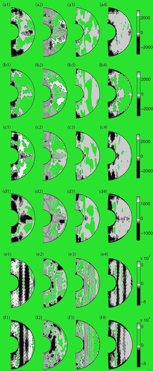
Axisymmetric power budget: for FFSF-21, FFNS-15, FTSF-15, FTNS-24, FTSF-20 and FTNS-33 dynamo models from the first to last row, respectively. The first, second, third and fourth columns show the time averaged axisymmetric ϕ components of the Lorentz, Coriolis, inertial and viscous terms, respectively. In these plots, red (blue) denotes sources (sinks) of power.
Axisymmetric power budget: for the FFSFC-16, FFNSC-14, FTSFC-09, FTNSC-08, FTSFC-13 and FTNSC-15 convection models with no magnetic field from the first to last row, respectively. The first, second, and third columns show the time averaged axisymmetric ϕ components of the Coriolis, inertial and viscous terms, respectively. In these plots, red (blue) denotes sources (sinks) of power.
The force balance can also be quantified by comparing the total forces over a volume integral in a spherical shell as employed by Soderlund et al. (2012). Fig. 11 shows the force integrals and their respective ratios as a function of Nu for the different boundary conditions employed. In these plots, we fix the parameters to E = 6 × 10− 5, RoM = 2 × 10− 5, qk = 1. In this parameter space the Coriolis force dominates all the models irrespective of the thermal or velocity boundary conditions. At Nu ≥ 8, the Lorentz force is balanced by the inertial force, that is the ratio of the Lorentz to inertial force is approximately 1. At Nu < 8, the Lorentz force does not seem to be balanced by either the Coriolis force or the inertial force. These results are in contrast to our Matching Coefficient study. This could be due to the fact that the Matching Coefficient only considers the ϕ component of the forces, or because the total force magnitude does not determine the force balance, and instead, a point-by-point comparison needs to be made (as is done with the Match Coefficient).
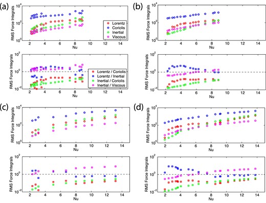
The rms force integrals: for models with E = 6 × 10⁻⁵, RoM = 2 × 10⁻⁵ and qk = 1. (a) FFSF, (b) FFNS, (c) FTSF and (d) FTNS. The top plots are the time averaged volume integrals of the rms Lorentz, Coriolis, inertial and viscous forces. The bottom plots are the time averaged ratios of the Lorentz force to the Coriolis and inertial forces, and the ratio of inertial force to Coriolis and viscous forces.
In Fig. 12, we only consider the ϕ component in the volume integrals. The degree of Lorentz–Coriolis balance seen in Fig. 8 is still not evident here, suggesting that total force magnitudes do not fully represent the force balances. Using Match Coefficients can better predict the force balance and the dipolarity of the field.
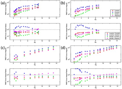
The rms force integrals of the ϕ component: for models with E = 6 × 10⁻⁵, RoM = 2 × 10⁻⁵ and qk = 1. (a) FFSF, (b) FFNS, (c) FTSF and (d) FTNS. The top plots are the time averaged volume integrals of the ϕ component rms Lorentz, Coriolis, inertial and viscous forces. The bottom plots are the time averaged ratios of the ϕ component of the Lorentz force to the Coriolis and inertial forces, and the ratio of inertial force to Coriolis and viscous forces.
3.5 Generation mechanisms
Fig. 13 presents these Match Coefficients as a function of Rol for different boundary conditions at fixed control parameters of E = 6 × 10− 5, RoM = 2 × 10− 5, qk = 1. At larger values of Rol, all of the models produce α2 dynamos. Intuitively, this is expected since a larger Rol implies a larger Ra and hence a stronger convective forcing. As Rol is decreased, the models with no-slip boundary conditions show a clear trend of increasing importance of ω effect and decreasing importance of α effect in generating the toroidal field. So the dynamo type in the no-slip models varies smoothly from αω to α2ω to α2 as Rol increases. The results for stress-free models are not as simple. At high Rol, the behaviour is similar to the no-slip models, but after Rol decreases to the point where the Match Coefficients of both effects are similar, the monotonic trends do not continue. There is large scatter in the Match Coefficient trends at lower Rol and it does not appear that the ω effect ever significantly dominates over the α effect. The stress-free dynamos, therefore, have either α2 or α2ω mechanisms.
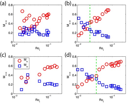
Match coefficient of α and ω effects versus local Rossby number: for models with E = 6 × 10− 5, RoM = 2 × 10− 5 and qk = 1. (a) FFSF, (b) FFNS, (c) FTSF and (d) FTNS. The green dotted line marks the transition of α effect dominance over ω effect.
Fig. 14 shows details of the field generation mechanisms. The time averaged toroidal magnetic field, creation of |$\skew3\vec{B}_T$|, and the creation of |$\skew3\vec{B}_T$| due to α and ω effects (terms in eq. 29) for models in order of increasing Rol, namely, FTNS-18, FTNS-22 and FTNS-32 are presented. It is evident that model FTNS-18 is an αω type dynamo, model FTNS-22 is an α2ω type dynamo and model FTNS-32 is an α2 type dynamo.
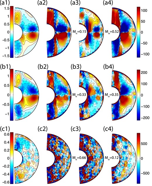
Dynamo creation mechanism: for models FTNS-18, FTNS-22 and FTNS-32 from first to last row, respectively. The first column shows the time averaged axisymmetric toroidal magnetic field. The second, third and fourth columns show the time averaged axisymmetric ϕ component of the total creation term of the toroidal magnetic field, toroidal magnetic field created by α effect and toroidal magnetic field created by the ω effect, respectively.
These results imply that axially dipolar dominated dynamos can be generated by α2, α2ω and αω mechanisms. In our models, all of the multipolar dynamos are generated by an α2 mechanism. This appears counterintuitive since the zonal flows in the high Rol models are stronger (see Fig. 6), however, as demonstrated in Fig. 9, the source of these strong zonal flows is the inertial force rather than the Coriolis force. It therefore appears that zonal flows must result from dynamos whose dominant force balance is between the Lorentz and Coriolis forces (rather than the Lorentz and inertial forces) to generate an axially dipolar dominated field in our models. These results also imply that the dominant Lorentz–Coriolis balance can occur with either generation mechanism for the toroidal field.
4 CONCLUSIONS
In this paper, we investigated the influence of different thermal and velocity boundary conditions on numerical dynamo models. We found that the resulting magnetic field morphologies most strongly depend on the local Rossby number (similar to previous work), but there are some secondary influences on the dipolarity of the field by the boundary conditions. Namely, at a given Rol, fixed temperature models are more dipolar than fixed flux models and stress-free models are more dipolar than no-slip models.
A single diffusivity-free scaling law for heat transport does seem feasible for all the dipolar models studied, although there is some variation among the different boundary conditions that may be important when extrapolating results of scaling laws to Earth-like parameters. The influence of different boundary conditions is particularly evident on Nu versus Ra/Rac scalings. Our multipolar models appear to obey different scaling laws from the dipolar models. Further investigation of scaling laws for multipolar models would benefit from a larger range in Ra, but this is numerically difficult presently.
The different scalings for multipolar and dipolar models is directly related to the different force balances in these models. Even though the magnetic energies of the dipolar and multipolar models were similar, dipolar models had a stronger degree of Lorentz–Coriolis balance whereas the multipolar dynamos possessed a dominant Lorentz-inertia balance. We demonstrated that plotting the axisymmetric Lorentz and Coriolis forces and estimating the Match Coefficient is a better way to establish the force balance than solely calculating the Elsasser number or comparing volume integrals of the forces.
We also demonstrated that a specific force balance does not imply a specific generation mechanism. A dominant Lorentz–Coriolis balance can be generated by either an α2, α2ω or an αω mechanism and result in dipolar dominated fields. In contrast, our multipolar fields, with dominant Lorentz-inertia balance, are all α2 type.
The authors thank U. Christensen and an anonymous reviewer for useful comments that improved this manuscript. S. Stanley acknowledges funding for this project by the Natural Sciences and Engineering Research Council of Canada (NSERC). Computations were performed on the gpc supercomputer at the SciNet HPC Consortium. SciNet is funded by the Canada Foundation for Innovation under the auspices of Compute Canada, the Government of Ontario, Ontario Research Fund – Research Excellence, and the University of Toronto.
REFERENCES
SUPPORTING INFORMATION
Additional Supporting Information may be found in the online version of this article:
Table S1. Dynamo model results.
Table S2. Results of convection models.
Table S3. Models without hyperdiffusion (Supplementary Data).
Please note: Oxford University Press is not responsible for the content or functionality of any supporting materials supplied by the authors. Any queries (other than missing material) should be directed to the corresponding author for the article.
