Resistivity structure underneath the Pamir and Southern Tian Shan

Abstract

1 INTRODUCTION

To understand the present state of the lithosphere, it is crucial to constrain the geodynamic processes governing intra-continental collision. The Pamir-Tian Shan region of Central Asia may be the best location to study these processes in situ. The mountain ranges and high plateau formed at the tip of the western Indian promontory through Cainozoic shortening of a magnitude similar to the adjacent Himalaya–Tibet system (e.g. Molnar & Tapponnier 1975; Schmidt et al.2011). The Tian Shan-Pamir-Hindu Kush orogen hosts some of the deepest active intracontinental subduction zones on Earth, connected with one of the most active areas of intermediate-depth seismicity (Chatelain et al.1980; Hamburger et al.1992; Burtman & Molnar 1993; Fan et al.1994; Pegler & Das 1998; Negredo et al.2007; Sippl et al.2013a). In addition, the orogen absorbs the highest strain rate over the shortest distance that is manifested in the India–Asia collision zone (Reigber et al.2001; Mohadjer et al.2010; Zubovich et al.2010; Ischuk et al.2013).

The multidisciplinary Tian Shan-Pamir Geodynamic Program (TIPAGE) addresses geodynamic questions related to intracontinental orogeny by combining numerical geodynamic modelling (part in Sippl et al.2013b), structural geology and geo-thermochronology (e.g. Schmidt et al.2011; Stübner et al.2013a,b; Stearns et al.2013), seismological investigations (e.g. Mechie et al.2012; Sippl et al.2013a,b; Schneider et al.2013), and a magnetotelluric (MT) survey in Kyrgyzstan and Tajikistan. The MT method is particularly sensitive to electrically conductive regions in the crust and upper mantle, which often imply the presence of fluids (Haak & Hutton 1986; Jones 1992). Fluids, their distribution with depth, and the temperature conditions are perhaps the most important controlling parameters for tectonic processes, as they dramatically influence the rheology of the crust and the style of deformation (e.g. Beaumont et al.2001; Klemperer 2006; Arora et al.2007; Rosenberg et al.2007). MT and seismological studies of active continental collision zones, such as the Himalaya–Tibet region or Anatolia, revealed mid crustal low resistivity/low velocity zones, which were interpreted as evidence for aqueous fluids and/or partially molten rocks (e.g. Berdichevsky et al.2010; review by Unsworth 2010; Xiao et al.2011). Some of these zones may accommodate flow of viscous crust over several hundreds of kilometres, causing crustal shortening and plateau growth (e.g. Clark & Royden 2000; Bai et al.2010). Fluid release due to metamorphism and its rheological consequences have been studied intensively in oceanic subduction regimes (e.g. Hacker 2008; Worzewski et al.2010; John et al.2012), however, eclogitization and associated fluid release play an equally important role in continental collision processes (e.g. Gao & Klemd 2001; Li et al.2004; Liou et al.2004; Jolivet et al.2005; Zheng 2012).

2 STRUCTURAL AND GEOLOGICAL SETTING

Prior to the India–Asia collision, distinct continental blocks collided with the southern margin of Eurasia, inheriting a lithological and structural fabric of about east–west trending microcontinents and sutures to the Cainozoic continental collision zone. By analogy with the adjacent Hindu Kush–Karakoram–Himalaya–Tibet orogen, the studied part of the Pamir features the following arcuate zones (Fig. 1; e.g. Vlasov et al.1991; Burtman & Molnar 1993; Schwab et al.2004; Schmidt et al.2011):

Figure 1.

Open in new tabDownload slide

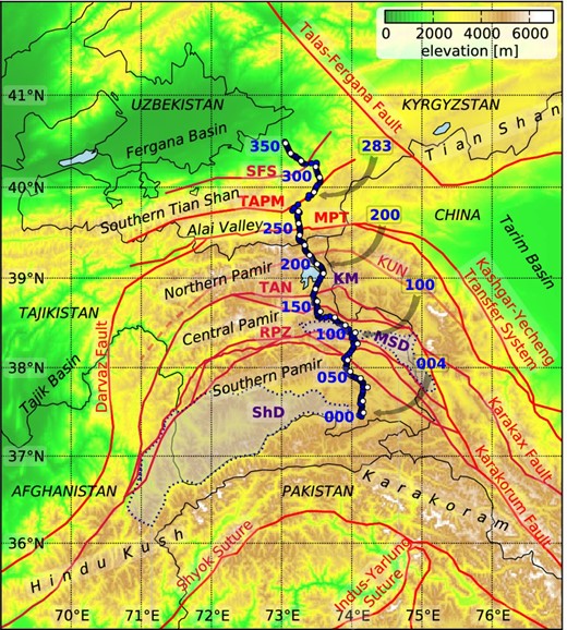
Map of the Pamir-Southern Tian Shan region. Blue and white circles indicate broad band and long period MT stations (in total 177 stations). Stations labelled 004, 100, 200 and 283 are discussed in detail in the text. The locations of major faults, sutures and gneiss domes are plotted with red and dashed lines (after Schwab et al.2004; Robinson et al.2007; Schmidt et al.2011; Lukens et al.2012). KM, Karakul-Mazar Unit; KUN, Kunlun Suture; MPT, Main Pamir Thrust; MSD, Muskol-Shatput Domes; RPZ, Rushan-Pshart Suture Zone; ShD, Shakhdara Dome; SFS, South Fergana Suture Zone;, Tanymas Suture Zone; TAPM, Turkestan-Alai Passive Margin.

The Northern Pamir stretches between the Tanymas Suture Zone in the south and the Alai Valley in the north. It contains the Palaeozoic–Early Mesozoic Kunlun magmatic arc and the Kunlun (Northern Pamir) Suture Zone in the north and the subduction-accretionary wedge of the Karakul-Mazar complex in the south; the latter corresponds to the Hoh Xil–Songpan-Ganze system of Tibet. In the Lake Karakul area, the Karakul-Mazar complex comprises thick, often graphite-bearing meta-sandstone and phyllite; a large part of it may be turbidite. Meta-siliciclastic and meta-volcanic rocks containing numerous ultramafic and mafic lenses (serpentinized peridotite, meta-gabbro, and meta-basalt) occur discontinuously in two zones. Permotriassic granitoids intruded the Karakul-Mazar complex.

The Central Pamir—between the Tanymas and Rushan-Pshart suture zones—comprises Palaeozoic–Jurassic platform rocks and relict Early Palaeozoic, mostly orthogneiss basement. Its central zone consists of Cainozoic high-grade metamorphic and minor igneous rocks, constituting the Muskol and Shatput domes (Schwab et al.2004; Schmidt et al.2011); these rocks exhumed at about 20–15 Ma from ∼30 km to upper crustal depths along normal-sense shear zones (Rutte et al.2013; Stearns et al.2013).

The Southern Pamir—south of the Rushan-Pshart Suture Zone—comprises the giant composite Shakhdara-Alichur crystalline Dome in the west and Late Palaeozoic–Mesozoic volcano-sedimentary strata in the east. The Shakhdara-Alichur Dome hosts Proterozoic gneiss, Palaeozoic–Mesozoic meta-sedimentary rocks, and massive Cretaceous and minor Palaeogene–Neogene granitoids (Schwab et al.2004; Schmidt et al.2011; Malz et al.2013; Stübner et al.2013a). The Cretaceous granitoids are part of the Andean-type arc built on the southern margin of Asia during the subduction of the Neo-Tethys oceanic lithosphere (Schwab et al.2004); the Cainozoic magmatism is mostly the product of regional anatexis (Schmidt et al.2011; Malz et al.2013). The Shakhdara Dome rocks, containing ubiquitous Cainozoic sills, dikes and migmatites, exhumed from ≥35 km to upper crustal depths at about 20–2 Ma along the crustal-scale, normal-sense, top-to-SSE South Pamir Shear Zone (Stübner et al.2013a,b). The eastern Southern Pamir also hosts crustal xenoliths that provided a record of metamorphism of 815–1100 °C at 60–100 km depth, mica-dehydration melting, and an average lower crustal geothermal gradient of ∼ 13 °C km⁻¹ prior and at their eruption at 11 Ma (Ducea et al.2003; Hacker et al.2005; Gordon et al.2012). The Cainozoic Pamir domes contain Barrovian-facies rocks recording peak metamorphic assemblages at about 750 °C and 0.75 GPa and geothermal gradients of 30–60 °C km⁻¹ in the upper 30–40 km of the crust during the Neogene; the Shakhdara Dome rocks were the hottest and are the most deeply and most recently exhumed. Numerous hot springs indicate a still enhanced geothermal gradient (Schmidt et al.2011; Stübner et al.2013a,b).

Sutures are zones of lithospheric weakness, which are prone to subsequent tectonic re-activation. The north-dipping Kunlun Suture Zone and the south-dipping Tanymas Suture Zone closed in the latest Palaeozoic–Early Mesozoic and the Rushan-Pshart Suture Zone closed in the Early Jurassic (Schwab et al.2004; Angiolini et al.2013). In the Pamir, the Kunlun Suture Zone constitutes the southern margin of the fold-and-thrust belt of the outer arc of the Pamir, which is about 25 km wide in the Alai Valley. The Tanymas Suture Zone comprises a Cainozoic backthrust (top-to-S) belt that emplaced Karakul-Mazar rocks onto the Central Pamir strata. The Rushan-Pshart Suture Zone also shows Cainozoic shortening, emplacing Southern Pamir rocks onto the Central Pamir sequences; steeply south-dipping reverse faults with a dextral oblique-slip component dominate this fold-and-thrust belt. The southeastern part of this belt transitions into the dextral strike-slip faults of the northeastern tail of the Karakoram Fault Zone; fault scarps and hot springs imply recent activity (Vlasov et al.1991, unpublished data of the TIPAGE project).

Since the onset of the India–Asia collision at about 50 Ma ago (e.g. Patriat & Achache 1984; Najman et al.2010; van Hinsbergen et al.2011a,b), the Pamir has accommodated about 600 km of crustal shortening (e.g. Burtman & Molnar 1993; Schmidt et al.2011), causing a doubling of its crustal thickness (60–75 km; Beloussov et al.1980; Mechie et al.2012; Schneider et al.2013). The whole Pamir has been moving northwards relative to the surrounding regions within the last 25 Ma (e.g. Sobel & Dumitru 1997; Sobel et al.2011), leading to overthrusting of the Tajik and Tarim Basins (Burtman & Molnar 1993). A remnant basin—the Alai Valley—links the Tajik Basin in the west and the Tarim Basin in the east (e.g. Burtman 2000; Coutand et al.2002). The system of faults along the Alai Valley's southern margin, the Main Pamir Thrust system (MPT), absorbs the main part of the present-day convergence between the Pamir and the Tian Shan (Mohadjer et al.2010; Zubovich et al.2010; Ischuk et al.2013). Sobel et al. (2013) described the MPT as currently mostly inactive, with much of the shortening accommodated along the Pamir Frontal Thrust system north of MPT. Here, we call the entire fold-and-thrust system at the northern margins of the Pamir as the MPT. Several authors (e.g. Burtman & Molnar 1993; Sobel et al.2013) interpreted this seismically active zone as the leading edge of the south-dipping intracontinental subduction of the crust of the Tajik-Tarim basins underneath the Pamir, whereas others (e.g. Sippl et al.2013b) suggested the involvement of most of the Tian Shan into the intracontinental subduction.

North of the Alai Valley and the Pamir arc, our profile crosses the Tian Shan, a Palaeozoic orogen, reactivated in the course of the India–Asia collision (e.g. Molnar & Tapponnier 1975; De Grave et al.2012). The Alai Range of the Southern Tian Shan consists mainly of Palaeozoic volcano-sedimentary rocks intruded by Devonian to Permian granitoids. The main tectonic structures in this part of the Tian Shan are the Turkestan-Alai Passive Margin and the South Fergana (or South Tian Shan) Suture Zone at the southern margin of the Fergana Basin; both zones were reactivated in the Cainozoic (e.g. Glorie et al.2011; De Grave et al.2012). The northernmost MT stations were located in the Fergana basin, a Cainozoic intramontane basin within the western Tian Shan orogenic system (e.g. Molnar & Tapponnier 1975; Coutand et al.2002).

3 MT DATA

3.1 Measurements

MT data were recorded in two field campaigns in 2008 and 2009 along a 350 km long, roughly north–south trending corridor from southern Tajikistan across the Pamir Plateau, the Alai Valley and the Southern Tian Shan to Osh in the Kyrgyz Fergana basin. In total, we recorded at 177 MT stations, whereof 26 combine broad band (BBMT, period range 10⁻³–10³ s) and long period recordings (LMT, 1–10⁴ s). The average station spacing was 2 km for BBMT sites and ∼14 km for combined BBMT+LMT sites. The overview map of the measurement area (Fig. 1) shows all TIPAGE MT stations as blue and white circles, indicating BBMT and LMT stations, respectively. At each of the MT stations, we recorded five channel electromagnetic data: two horizontal magnetic and electric field components and the vertical magnetic field. Recording times were at least 3 days for sites with BB data and ∼2 weeks for sites with LMT data. We used GPS synchronized S.P.A.M. MkIII broadband instruments (Ritter et al.1998) and Earthdata loggers for data recording and non-polarizable Ag/AgCl telluric electrodes for electric field measurements. For broad band measurements of magnetic fields, we used Metronix MFS05 and MFS06 induction coil magnetometers and Geomagnet fluxgate magnetometers for long period recordings. In the sparsely populated Pamir Plateau region, data quality is excellent. These stations were processed by applying robust single-station processing algorithm. Anthropogenic electromagnetic noise affected the data of a number of stations in the Tian Shan; these data required reprocessing using the remote reference processing technique. Therefore, we took advantage of simultaneously operating sites in Kyrgystan and Tajikistan, which where separated by ∼50–100 km, so we often had multiple remote reference site options. We used the robust, remote-reference EMERALD data processing package (Ritter et al.1998; Weckmann et al.2005; Krings 2007) to compute impedance tensor and vertical magnetic transfer function data.

3.2 Dimensionality and Regional Strike

For geoelectric strike analysis, we applied the method of Becken & Burkhardt (2004). The rose diagram in Fig. 2a shows the regional geoelectric strike when analyzing the longer period data between 10 and 10 000 s of all stations. The geoelectric strike direction has a principal 90° ambiguity, which can be resolved by examining in addition the vertical magnetic field transfer functions (induction vectors, Fig. 2b). The period range under consideration corresponds very roughly with middle to lower crustal levels or even below (∼10–100 km). The average strike direction of WSW–ENE (75°) is consistent with the structural trend of the area (e.g. Schwab et al.2004). A well defined and consistent geoelectric strike direction is prerequisite for later 2-D interpretation of the data. Fig. 2(c) provides information about the spatial distribution and consistency of geoelectric strike directions for a range of periods and for different profile segments. As expected, this compilation exhibits generally larger variability for the strike directions. At shorter periods (0.1–100 s), which correspond roughly to induction volumes of a few hundred meters to a few kilometres, scattering strike directions may indicate local 3-D or 1-D conditions for which strike is undetermined. For longer periods (10–10 000 s), we observe more uniform geoelectric strike directions along the profile, which are generally consistent with the overall WSW–ENE direction obtained for all sites. For all subsequent 2-D inversions, we therefore rotated the impedance tensors to make the x-axis point WSW (255°) parallel to the main current flow and the y-axis roughly parallel to the station line in a NNW (345°) direction. The skewness of the impedance tensor is a non-dimensional rotationally invariant parameter to characterize the complexity of subsurface structures (Bahr 1988). For 1-D or 2-D conductivity distributions, skewness values are 0. Non-zero values indicate the presence of 3-D structures but practically, values of 0.2–0.3 are considered still compatible with 2-D assumptions. Pseudo-sections of the skewness in Fig. 3(a) show values below 0.2 for most stations and periods. Fig. 3(b) shows the distribution of skewness values. In total 73 per cent of our data exhibit skewness values below 0.2, only 8 per cent of the data are above 0.3. Skewness values >0.3 occur at stations 70–90 for longer periods, where we also observe phases >90°. Clearly, we cannot expect explaining all aspects of these high quality data with 2-D modelling, but the majority of the data is consistent with 2-D assumptions. The large skewness values observed towards the northern end of the profile, however, are predominantly caused by high levels of anthropogenic noise.

Figure 2.

Open in new tabDownload slide

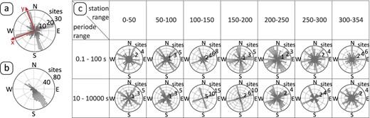
(a) Regional strike analysis of all stations using a wide period range between 10 and 10 000 s. The rose diagrams show the number of stations with a certain regional strike direction (after Becken & Burkhardt 2004). The final coordinate system for rotating the MT data into TE and TM modes is marked by red arrows. (b) Rose diagram of induction vector directions (Wiese convention) of all stations and the period range between 10 s and 10 000 s. With the induction vectors, the principal 90° ambiguity in diagram (a) can be resolved. (c) Regional strike examination similar to (a) but now analysing subsets of the data. Strike directions for various period (rows) and station ranges (columns) show larger variability but generally consistency with the overall strike direction; longer periods correspond to larger induction volumes.

Figure 3.

Open in new tabDownload slide

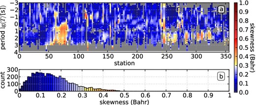
(a) Pseudo-sections of skewness after Bahr (1988). (b) Distribution of skewness values. 73 per cent of our data show skew values below 0.2 (blue colours), which are generally considered compatible with a 2-D assumption. At stations 070–090 and some sites between 260 and 340 we observe higher skewness values for longer periods, which are indications for an influence of 3-D structures or anthropogenic noise.

3.3 2-D Inversion

To solve the 2-D MT inverse problem, we used an algorithm based on a regularized, nonlinear conjugate gradients (NLCG) scheme (Rodi & Mackie 2001), implemented in the WinGLink software package (version 2.20.09). Fig. 4 shows our preferred 2-D model. For the 2-D inversion, all station locations were projected onto a line perpendicular to the determined geoelectric strike direction (parallel to the y-axis in Fig. 2a), roughly connecting the first and the last station of the profile (compare to map in Fig. 1); the 2-D topography along the profile is considered. We used the following settings for the inversion: joint inversion of TE+TM+Hz mode, 189 × 798 cells, τ = 30, ρ_start = 100 Ωm, weighting: α = β = 1, H = V = 500, error floors: Δρ_TE = 1000 per cent, Δφ_TE = 1.45°, Δρ_TM = 30 per cent, Δφ_TM = 1.45°, ΔT_Y = 0.05. We set the error floors to emphasize fitting the phases, which are not affected by static shift, and down-weighting apparent resistivities. Particularly, |$\rho _{\text{TE}}$| with an error floor of 1000 per cent was effectively excluded from the inversion. Prior to the inversion, we removed data points obviously disturbed by noise (grey areas in data pseudo-section of Fig. 6a), but we did not apply additional smoothing. Fig. 4 shows the result of a joint inversion of the TE and TM mode impedances and the vertical magnetic field (T_Y component).

Figure 4.

Open in new tabDownload slide

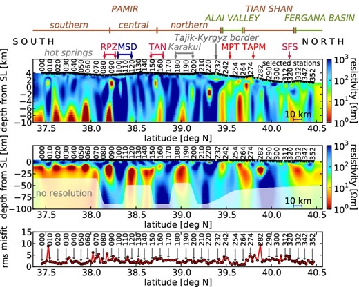
2-D inversion result, using TE and TM mode impedances and vertical magnetic transfer functions, truncated at depths of 10 km (upper plot) and 100 km (middle diagram). Unresolvable zones in the model are marked with a grey ‘no resolution’ area. Please note the horizontal scale bar in the lower right corner of each plot. The vertical exaggeration of the upper plot is ∼1:4.3, of the lower diagram ∼1:0.6. Arrows above the plots indicate locations of major geological features (see Fig. 1 for abbreviations). The rms misfit values for each station are plotted at the bottom. Zones of low resistivity (high conductivity) are shown in yellow and red colours.

where c indicates a data component (e.g. ρ_TE, φ_TE, ρ_TM, φ_TM), |$d_{i}^{\: c, {\rm obs}}$| and |$d_{i}^{\: c, {\rm calc}}$| are the observed (measured) and calculated (model response) data points, with i indicating period. n_c is the number of data points for component c (e.g. number of periods), Δ_c the estimated error for the component c and rms_tot the total rms misfit value.

To probe the robustness of the inversion result, we varied systematically a wide range of inversion parameters, including the starting model, grid size, frequency range, error floors and data weighting. An important aspect of this particular inversion scheme is finding the most appropriate smoothness (regularization) parameter τ. Plotting the model roughness versus the rms misfit of the inversion results with different settings of the smoothing parameter yields the so-called ‘L-curve’, a Pareto-Optimal Front. The best value of τ is found near the kink of the L-curve as an optimum trade-off between model roughness (keeping structures coherent) and data misfit; for the model in Fig. 4, we found an optimum τ = 30. Due to grid-size restrictions of the WinGlink software package, we had problems inverting all 177 stations at all frequencies (1000 to 0.0001 Hz) and considering topography. Therefore, we obtained the model in Fig. 4 by combining five independent 2-D inversion results, each including only a subset of ∼35 stations. To create a consistent and smooth combination of these models, we first ensured that their vertical grid spacings were the same. Subsequently, the models were stitched together at the positions of the last and first stations of any two consecutive models. Fig. 5 demonstrates this approach. It shows one stitched interim section at ∼38.6°N (stations 128–150). As can be expected, the individually inverted 2-D sections do normally not match, revealing sometimes sharp resistivity contrasts where the profiles were stitched together (Fig. 5a). To smoothen these contrasts, we (re-)imported the stitched model sections around the stitching line into WinGLink and applied ∼20 additional inversion iterations, using the same settings as before (Fig. 5b). The inversion was restarted but only the transitional segment between any two interim sections was allowed to change. Thereby we could ensure smooth and continuous transition between the segments with similar data fit as for the individual inversions. The final smooth section in Fig. 4 was achieved by combining five of these individually obtained inversion sections. This allowed us to set-up a very dense grid (in total ≈800 horizontal cells × 200 vertical cells), which facilitated good sampling of vertical topography gradients and smooth lateral conductivity variations in the upper crust (final model in Fig. 4). We performed a variety of resolution and sensitivity tests, for example, by removing or manipulating prominent structures of the model and re-running the inversion and/or comparing forward responses of the manipulated model with the prior model. Thus determined unresolvable zones in the model are marked with a grey ‘no resolution’ area in Fig. 4.

Figure 5.

Open in new tabDownload slide

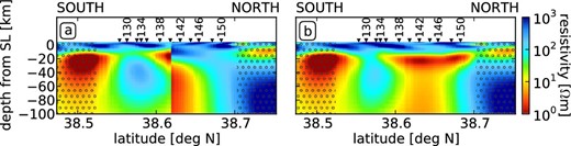
The example illustrates how independently inverted 2-D sections were stitched together. (a) Two independently inverted sections are combined where they overlap between stations 138 and 142. Obviously, the two individual inversion models do not match at their edges (the stitching line). Subsequently, regions far away from the stitching line were locked (dotted) and the inversion was re-started. (b) The figure on the right hand side shows the final stitched inversion result after 20 iterations.

Fig. 6 shows pseudo-sections of measured data (6a) and inversion results (6b). The data fit can be examined in more detail in Figs 7(a) and (b) with pseudo-sections of total differences between observed and calculated data and pseudo-sections of rms values. Fig. 7a shows the total differences between observed and calculated data points, colour-coded and displayed for each component, period and station. In Fig. 7(b) pseudo-sections of rms values for each component are plotted. The rms plots were derived from the absolute misfits by weighting the misfit values with the estimated error floors. Areas with intense blue or red colours in Figs 7(a) and (b) indicate poorly fitted data. Less saturated colours indicate that the TM mode apparent resistivity and phases (‘rho TM diff’ and ‘phi TM diff’) are better fitted then the TE mode data. Fitting the TE mode is difficult with 2-D inversion as ρ_TE is often affected by static shift, which can be seen in Fig. 7(a) by stripes in the misfit plots (‘rho TE diff’). The misfit plots of the TE phase ‘phi TE diff’ also exhibits regions with intense colours, where the absolute misfit is in the range of 15–20°. Comparison of all rms pseudo-sections in Fig. 7(b) reveals that the φ_TE plot (‘phi TE RMS’) shows the largest misfits and therefore, this component dominates the total rms. Nevertheless, the data fit of φ_TE is still acceptable. Fig. 8 shows observed and predicted data curves for four selected stations along the profile (004, 100, 200, 283). The diagram gives an indication of the generally high data quality. TM mode apparent resistivities and phases are well reproduced by the model predictions, but also TE mode components and vertical magnetic transfer functions are reasonably well fitted.

Figure 6.

Open in new tabDownload slide

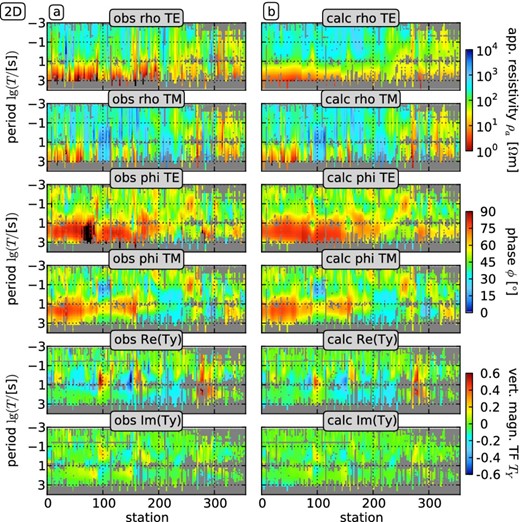
(a) Observed and (b) calculated (2-D model response, Fig. 4) pseudo-sections of apparent resistivity ρ, TE and TM mode (‘rho TE/TM’), phase φ, TE and TM mode (‘phi TE/TM’) and vertical magnetic transfer functions T_Y, real and imaginary part (‘Re(Ty)/Im(Ty)’). The calculated data are the forward responses of the 2-D model shown in Fig. 4. Grey areas indicate noisy data points, which were removed prior to inversion. For station locations see Fig. 1.

Figure 7.

Open in new tabDownload slide

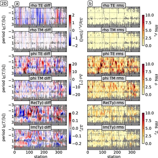
(a) Pseudo-sections of the absolute data misfit of the 2-D model (Fig. 4), that is the total difference between observed and calculated data points, colour-coded for each component, period and station. (b) The rms values for each component, period, and station, calculated and displayed as pseudo-sections.

Figure 8.

Open in new tabDownload slide

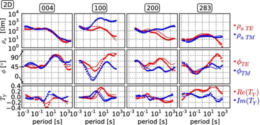
Measured (dots) and calculated (lines) transfer functions from the 2-D model for four representative stations from different profile regions (sites 004, 100, 200, 283). All data are shown in rotated coordinates. Red colours show the TE mode apparent resistivity and phase curves and the real part of the vertical magnetic transfer function. Blue curves show the TM mode apparent resistivity and phase curves and the imaginary part of the vertical magnetic transfer function. The four stations are marked with black arrows in Fig. 1.

3.4 3-D Inversion

For 3-D MT inversion, we used the code of the Modular Electromagnetic Inversion System (ModEM: Meqbel 2009; Egbert & Kelbert 2012). This package includes a parallelized gradient-based frequency-domain inversion code for 3-D MT data. In order to optimize computing time, we used only every second period. A joint inversion of all impedance components and the vertical magnetic transfer functions converged after 40 iteration to the model displayed in Figs 9 and 10. We used relatively strong horizontal and vertical smoothing (smoothing parameter of 0.4). Error-floor settings were 5 per cent for off-diagonal impedance elements, 10 per cent for diagonal impedance elements and 5 per cent for vertical magnetic transfer functions. The a priori and starting model was a homogeneous half space with ρ_start = 100 Ωm. We used a dense grid of 260 × 100 × 60 cells with a lateral cell size of 1.4 km × 1.4 km for the main inner part of the model and larger cells towards the model edges. Cell thicknesses of the uppermost layer are 30 m, increasing with depth by a factor of 1.2.

Figure 9.

Open in new tabDownload slide

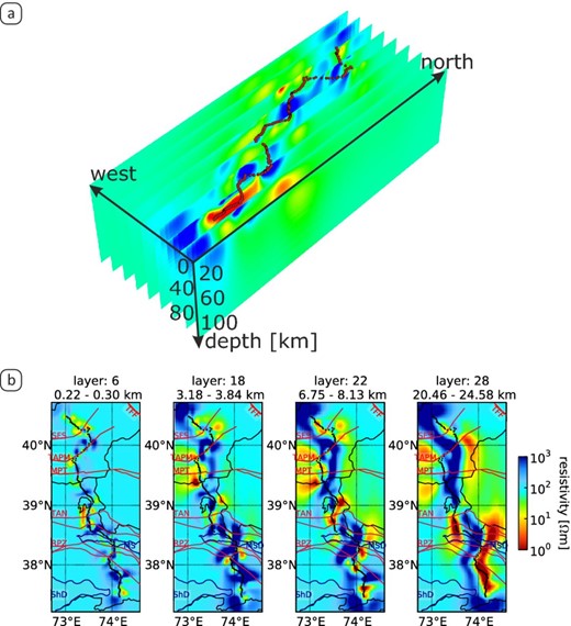
3-D inversion results from joint inversion of all impedance components and the vertical magnetic transfer functions, using the ModEM 3-DMT code (Meqbel 2009; Egbert & Kelbert 2012). (a) Overview plot of the 3-D model, showing vertical north–south slices through the model and station locations at surface. (b) Horizontal slices through the model at different depths, with projected geological boundaries (red lines), political borders (black lines) and station locations (chain of black dots). Note the inversion generates structures predominantly near stations, which are aligned along a profile (corridor). The peripheral zones of the model remain unchanged from the 100 Ωm starting model. For abbreviations see Fig. 1.

Figure 10.

Open in new tabDownload slide

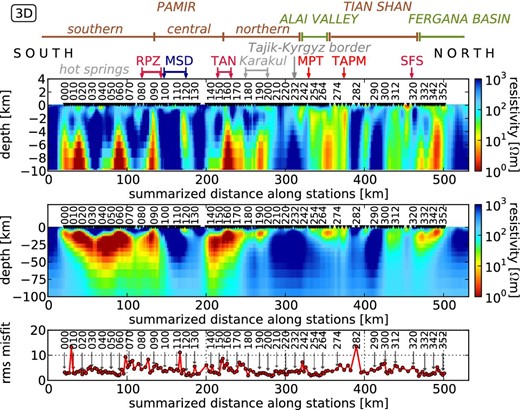
Vertical cross sections (10 and 100 km depths) of the 3-D model, approximately following the crooked station line. The units of the horizontal axes are given in kilometres, as summed up distances between stations. Resistivity values were taken from a column underneath a station or following a straight line between any two stations. The vertical exaggeration of the upper plot is ∼1:9, of the lower plot ∼1:0.9. Arrows above the plots indicate locations of major geological features (see Fig. 1 for abbreviations). The plot at the bottom shows rms misfits for each station, calculated using the formula in Section 3.3. The rms values here can be directly compared with those of and in Fig. 4, as the same error settings and formulas were used for the rms calculations. Comparing this plot to the result of the 2-D inversion in Fig. 4 shows that the main resistivity features are robust as they appear in the 3-D and 2-D calculations.

We applied the same data rotation for 3-D inversion as for the 2-D inversion. Thus, the off-diagonal (xy and yx) impedance components (Fig. 11a) correspond directly to the TE and TM mode data of the 2-D case, as can be seen by comparing Figs 7(a) and 11(a). The forward responses of this 3-D model are shown as pseudo-sections in Fig. 11(b). Figs 12(a) and (b) show in analogy to Fig. 7 pseudo-sections of the total differences between observed and calculated data and pseudo-sections of rms values. In Fig. 13, we plot observed data and 3-D model responses of all used data components for selected sites 004, 100, 200 and 283. The total rms misfit calculated with ModEM is 4.5. Using the same calculation and assuming for the 3-D model the same error settings as for the 2-D model, we obtained an rms of 3.9 for the 3-D model. This value can be directly compared to the 2-D rms of 2.7. Note that the ModEM package fits impedances and not apparent resistivity and phases. Therefore, the influence of static shift could not be as in 2-D reduced by down-weighting apparent resistivity, which leads to a slightly better data fit of the apparent resistivities in 3-D than in 2-D, but to a worse fit of the phases [see apparent resistivity and phase misfit pseudo-sections in Fig. 7a (2-D) and in Fig. 12a (3-D)]. The data fit of the vertical magnetic transfer functions is generally poor in the 3-D model (see T_X and T_Y misfit and rms pseudo-sections in Fig. 12). For better comparison of 2-D and 3-D models, we created a cross section through the 3-D model following a bended line along the station locations at surface (Fig. 10). Comparison of this 3-D model cross section with the 2-D model in Fig. 4 shows that all important structures of the well-tested 2-D model are reproduced by the 3-D inversion (and vice versa). The horizontal axes in Fig. 10 are in kilometres, as summed up distances between stations along the bended profile line. For better comparison with the 2-D model in Fig. 4, please use station numbers and indicated geological features (above the diagrams). We have not performed as exhaustive model testing of the 3-D model as we did for the 2-D models, as this is extremely time consuming. Since the station distribution along a single line (or corridor) is far from being ideal for 3-D inversion, we do not discuss 3-D structures in detail, but rather use the 3-D inversion result as confirmation for the validity of the 2-D approach.

Figure 11.

Open in new tabDownload slide

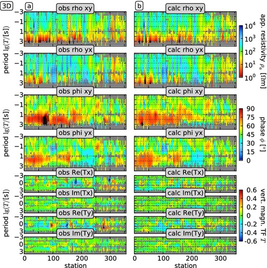
(a) Observed and (b) calculated (3-D model response, Figs 9 and 10) pseudo-sections of apparent resistivity ρ, TE and TM mode (‘rho TE/TM’), phase φ, TE and TM mode (‘phi TE/TM’) and vertical magnetic transfer functions T_Y, real and imaginary part (‘Re(Ty)/Im(Ty)’). The calculated data are the forward responses of the 2-D model shown in Fig. 4. Grey areas indicate noisy data points, which were removed prior to inversion.

Figure 12.

Open in new tabDownload slide

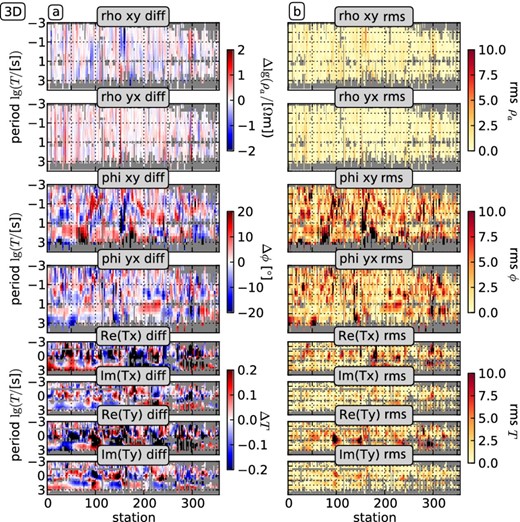
(a) Pseudo-sections of the absolute data misfit of the 3-D model, that is the total difference between observed and calculated data points, colour-coded for each component, period and station. (b) The rms values for each component, period and station, calculated and displayed as pseudo-sections. We calculated the rms value using the same error estimations in 3-D as in 2-D, thus pseudo-sections can be directly compared to the 2-D result in Fig. 7(b). For station locations see Fig. 1.

Figure 13.

Open in new tabDownload slide

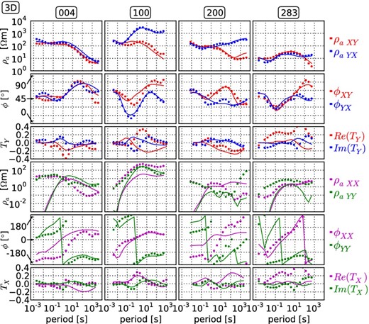
Measured data (dots) and 3-D responses (lines) for four representative stations from different profile regions (sites 004, 100, 200, 283; same as in Fig. 7). Apparent resistivity ρ_a and phase φ, calculated from off-diagonal (‘XY’ and ‘YX’) and diagonal (‘XX’ and ‘YY’) impedance-tensor elements, and vertical magnetic transfer functions T_X and T_Y, real and imaginary part. Black arrows in Fig. 1 highlight the station locations.

4 DISCUSSION

The 2-D (Fig. 4) and 3-D (Figs 9 and 10) inversion results reveal very similar overall resistivity structures for the upper and middle crust along the profile. The upper crust in the Pamir is generally resistive but separated by a number of subvertical conductive zones; some almost reaching surface. The middle and lower crust of the Southern and Central Pamir reveals laterally extended highly conductive regions. The Alai Valley is electrically conductive at all crustal levels, with higher resistivities in the middle crust. The generally resistive Southern Tian Shan features conductive anomalies at its southern and northern slopes, cutting through the entire crust.

4.1 Additional geophysical data

For the interpretation of the resistivity model we refer mostly to the 2-D inversion results of Fig. 4. It is useful, however, to include additional information from other accompanying geophysical experiments carried out within the framework of the TIPAGE project (see Figs 14a–d).

Figure 14.

Open in new tabDownload slide

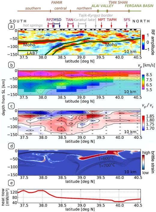
Additional geophysical and geological information from accompanying TIPAGE experiments. Arrows above the diagram indicate locations of the major geological structures. RPZ, Rushan-Pshart Suture Zone; MSD, Muskol-Shatput domes; TAN, Tanymas Suture Zone; MPT, Main Pamir Thrust; TAPM, Turkestan Alai passive margin; SFS, South Fergana Suture Zone (locations after Schwab et al.2004; Robinson et al.2007; Schmidt et al.2011; Lukens et al.2012, see also Fig. 1). (a) Receiver function cross section modified from Schneider et al. (2013). Green lines highlight the main seismological discontinuities of the lithosphere and a converter pair associated with the south-dipping intracontinental subduction zone underneath the Pamir. (b) Absolute P-wave velocity along 73.5°E (modified from Sippl et al.2013b). (c) v_p/v_s ratio along 73.5°E (modified from Sippl et al.2013b). (d) Thermomechanical model of the Pamir-Tian Shan zone (from Tympel and Sobolev, description in Sippl et al.2013b). Colour codes indicate the amount of brittle strain. Solid black lines show temperature isolines between 600 and 700 °C. (e) Heat-flow distribution along the MT profile line (from Duchkov et al.2001).

A set of 110 seismological stations distributed over Tajikistan and southern Kyrgyzstan recorded teleseismic events and local seismicity for 2 yr (Schneider et al.2013; Sippl et al.2013a,b). 58 of these stations gathered data along the MT profile. Receiver function analysis (Schneider et al.2013, Fig. 14a) revealed a Moho depth of ∼70 km depth beneath the Pamir and at ∼45 km depth beneath the northern edge of Southern Tian Shan. A prominent seismic converter, dipping southward underneath the Northern and Central Pamir, was interpreted by Schneider et al. (2013) as south-dipping subduction of lower continental crust and lithospheric mantle of the Alai Valley and Southern Tian Shan underneath the Pamir. Figs 14(b) and (c) show absolute P-wave velocities and v_p/v_s ratios along 73.5°E derived from local earthquake tomography (modified after Sippl et al.2013b). The most prominent crustal anomaly revealed by these data is a low velocity zone in the southern Pamir starting at a depth of ∼15 km, with v_p as low as 5.5–5.7 km s⁻¹ (Fig. 14b) and high v_p/v_s ratios in the middle crust south of 38°N (Fig. 14c, see also Sippl et al.2013b).

A series of N–S oriented 2-D thermomechanical cross section models were computed by Tympel and Sobolev to study the influence of rheological and compositional parameters during the India–Eurasia collision (published in Sippl et al.2013b). Fig. 14(d) shows a snapshot of accumulated strain overlain by temperature isolines. Focusing on the evolution of the Central Pamir, the Alai Valley, and the Tian Shan, a finite element code (SLIM3-D/2-D; Popov & Sobolev 2008) was used, which can simulate elasto-visco-plastic rheology, generate self-consistent faults, incorporate free surface boundary conditions and is equipped with routines to model phase transformations in crustal rocks. From the resulting models a successful candidate was selected which provided good agreement with other TIPAGE observations, such as a southerly dipping and steepening (‘rollback’) slab of Eurasian origin (Schneider et al.2013) which occurs in the models due to the force exerted by the high topography of the Pamir plateau.

Fig. 14(e) shows surface heat flow along our profile, following observations by Duchkov et al. (2001). Surface heat flow along our profile exceeds 120 mW m⁻² in its southern part but rapidly drops to below 80 mW m⁻² between 38.1°N and 38.3°N (Fig. 14e). The region of elevated heat flow coincides with the occurrence of up to a dozen hot springs, mapped in the Shakhdara-Alichur Dome of the Southern Pamir (Stübner et al.2013a). The heat source could be a combination of intracrustal heating (as reported for the Himalayan geothermal belt by Hochstein & Regenauer-Lieb 1998), mantle upwelling with delamination of lower crust (as modelled by Tympel and Sobolev in Sippl et al.2013b), or asthenosphere rise due to a slab break-off (e.g. Mahéo et al.2002; Stearns et al.2013).

Similarly elevated surface heat flow was reported from western China (Wang 2001; Tao & Shen 2008). It is possible, that the area of high heat flow in the Southern Pamir is connected with the Himalayan geothermal belt (Hochstein & Regenauer-Lieb 1998), a system of circulating geothermal fluids associated with heat generation by plastic deformation north of the India–Asia collision front.

4.2 Migmatization and magmatism and/or crustal flow beneath the Southern Pamir

Fig. 15 shows a compilation of the 2-D resistivity structures and the most important features derived from seismology: the Moho and the south-dipping converters (Schneider et al.2013) and the earthquake locations (Sippl et al.2013a). Conductor C1 in the Southern Pamir, located beneath an ∼10-km-thick resistive upper crust (resistor R1), is the most prominent and robust feature of the MT inversion models (Fig. 15). It captures the area south of the Rushan-Pshart Suture Zone, possibly extending further south into the Wakhan corridor of Afghanistan. The high conductivity begins at upper-crustal depths (∼10–15 km). Due to the high attenuation of electromagnetic fields in conductive layers, the lower boundary of the conductor C1 is not resolved. It is possible, though, that the high conductivity region of C1 reaches lower crustal or even mantle depths. The resistivity values of this zone are below 1 Ωm between 37.88°N and 38.00°N (stations 046–070), below 3 Ωm between 37.55°N and 37.75°N (stations 012–030) and below 5 Ωm for the entire area between 37.55°N and 38.00°N (stations 010–070). What are the causes of these remarkably low resistivities in the middle crust: melts, aqueous fluids, or a combination of both?

Figure 15.

Open in new tabDownload slide

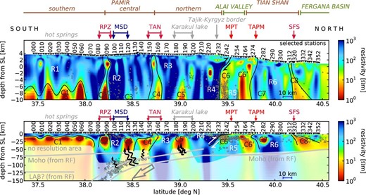
2-D resistivity model truncated at depths of 10 and 150 km. Please note the horizontal scale bar in the lower right corner of each plot. The vertical exaggeration of the upper plot is ∼1:3.7, of the lower plot ∼1:0.4. Grey lines indicate seismic converters derived from receiver function analysis (Schneider et al.2013). Circles mark earthquake locations (Sippl et al.2013a). Black lines and abbreviations: C, conductor; R, resistor; RPZ, Rushan-Pshart Suture Zone; MSD, Muskol-Shatput Domes; TAN, Tanymas Suture Zone; MPT, Main Pamir Thrust; TAPM, Turkestan Alai Passive Margin; SFS, South Fergana Suture Zone (locations after Schwab et al.2004; Robinson et al.2007; Schmidt et al.2011; Lukens et al.2012, see fig. 1).

Local earthquake tomography (Sippl et al.2013b) revealed a low velocity zone in the middle crust of the Southern Pamir (Fig. 14b). Relatively low v_p/v_s ratios occur in the upper crust and high v_p/v_s values in the middle crust (Fig. 14c). High temperatures at mid-crustal levels, which are predicted by the thermo-mechanical modelling (published in Sippl et al.2013b, Fig. 14d), coincide with the region of the Southern Pamir. This particular temperature distribution is a very robust feature of the model. In agreement to the modelling results, Duchkov et al. (2001) found high surface heat flow, exceeding 120 mW m⁻² in the Southern Pamir (Fig. 14e). Assuming a thermal conductivity of ∼2.5 W (m·K)⁻¹ (which are typical for crustal materials, e.g. Hochstein & Regenauer-Lieb 1998; Duchkov et al.2001; Wang 2001; Vermeesch et al.2004), a heat flow of 120 mW m⁻² implies a thermal gradient of ∼50 °C km⁻¹. Therefore temperatures of 600–700 °C should occur at depths of 12–14 km, roughly coincident with the depth to the top of C1. For Southern Tibet, the 600 °C isotherm was proposed for at a depth of 18 km (Mechie et al.2004). Temperatures between 600 and 700 °C coincide approximately with the melting point of wet felsic crust (Hyndman & Hyndman 1968; Schmeling 1986; Li et al.2003; Bürgmann & Dresen 2008).

Remarkably similar low resistivity–low velocity zones in the middle crust associated with elevated surface heat flow were discovered at a number of places beneath Central and Southern Tibet (e.g. Unsworth 2010). The interpretation of these zones is still under debate; possible explanations include melts (Pham et al.1986; Nelson et al.1996), aqueous fluids (Makovsky & Klemperer 1999) and a combination of both (Li et al.2003). Explaining the Southern Pamir conductor solely with free aqueous fluids seems difficult though. Firstly, temperatures within the bright spots in C1 (Fig. 15) would have to be below the wet granite solidus at approximately 650 °C, which would imply surface heat-flow values below 100–110 mW m² (Makovsky & Klemperer 1999). Secondly, crustal seismicity in the Southern Pamir is sparse and occurs only in the upper crust, that is above conductor C1 (see earthquake occurrences of Sippl et al.2013a, in Fig. 15). All of these observations support ductile deformation for the region of C1. P-T conditions consistent with large amounts of saline water, however, would be more associated with brittle deformation (Bürgmann & Dresen 2008).

where σ₁ and σ₂ indicate electrical conductivities of the fluid and the rock matrix, respectively.

Figs 16(a) and (b) show bulk conductivities for Archie's law for two different exponents m (0.9 and 1.4), two different assumptions for σ₁ (1 and 5 S m⁻¹) and three values for σ₂ (0.01, 0.001 and 0.0001 S m⁻¹). Note, for this range of parameters, there are hardly any differences between the classical Archie's law (Archie 1942) and the modifications by Glover et al. (2000). The green lines in Figs 16(a) and (b) are calculated using Archie's empirical interconnectivity exponent m = 0.9, which corresponds to a highly interconnected fluid phase. Red lines, with a corresponding exponent m = 1.4, describe less interconnected fluids. In Fig. 16(a), solid lines were calculated assuming a conductivity of σ₁ = 5 S m⁻¹ (0.2 Ωm) for the fluid phase, dashed lines represent fluid conductivities of σ₁ = 1 S m⁻¹. In Fig. 16(a), we assume matrix conductivity of σ₂ = 0.001 S m⁻¹ (1000 Ωm), while σ₂ was varied in Fig. 16(b) in a range from 0.0001 to 0.01 S m⁻¹ (100–10 000 Ωm). For Fig. 16(b), the matrix conductivity σ₂ hardly influences the total bulk conductivity of the mixed system.

Figure 16.

Open in new tabDownload slide

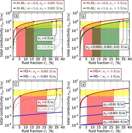
Total bulk conductivity σ_tot versus fluid fraction C₁ in a system of two phases with different conductivities σ₁ and σ₂, for example a rock matrix and a fluid phase, assuming different mixing laws and parameters. Marked in yellow are bulk conductivities in a range from 0.2 to 1 S m⁻¹ (1 to 5 Ωm), as observed for the mid-crustal conductor C1 in the Southern Pamir. Green and red areas mark the percentage of fluids or melts required to explain the observed bulk conductivities of 0.2–1 S m⁻¹ with different mixing law assumptions. (a, b) m.AL: modified Archie's law, adjusted for two conducting phases by Glover et al. (2000) for two different interconnectivity exponents m (0.9, green and 1.4, red), two different assumptions for σ₁ in diagram a (1 S m⁻¹, dashed and 5 S m⁻¹, solid) and three values for σ₂ in diagram b (0.01, 0.001 and 0.0001 S m⁻¹). (c, d) Upper and lower Hashin-Shtrikman bounds (HS+ and HS–; red and blue lines; Hashin & Shtrikman 1962, 1963; Waff 1974) for a system with a fluid conductivity σ₁ of 5 and 1 S m⁻¹ and rock matrix conductivity σ₂ of 0.001 S m⁻¹ (diagram c), and varying rock matrix conductivity 0.0001 S m^-1 < σ₂ < 0.01 S m⁻¹ (diagram d).

The parts coloured in yellow in all plots of Fig. 16 mark the conductivity range of 0.2 to 1 S m⁻¹ (1 to 5 Ωm), which corresponds to our observations. As described above, the Southern Pamir mid-crustal conductor C1 in its entirety has conductivities above 0.2 S m⁻¹ (resistivities below 5 Ωm, compare to Fig. 15), in some parts even exceeding 1 S m⁻¹ (1 Ωm, between 37.88°N and 38.00°N, stations 046–070).

Assuming a fluid with a conductivity of 5 S m⁻¹ (resistivity 0.2 Ωm) and using Archie's law to explain a bulk conductivity of 1 S m⁻¹, about 17 per cent of highly interconnected fluids would be required to explain the observations in some of the inner parts of conductor C1 (right side of red area in Fig. 16). For the entire volume of high conductivity, at least 3 per cent of perfectly interconnected fluids or 10 per cent less interconnected fluids are required by Archie's law (left sides of red and green areas in Fig. 16a). Using the upper Hashin-Shtrikman bound for modelling the fluid content yields about 6 per cent for the entire volume of C1 and about 27 per cent for the most conductive parts (Fig. 16c). Values above ∼20 per cent partial melting or fluid content are considered unrealistically high because melt or fluids would start to migrate. An interconnection exponent m = 0.9 for Archie's law seems more appropriate to describe the fluid fraction of the Southern Pamir mid-crustal conductor. This assumption leads to fluid fractions of at least 3 per cent for the entire conductive zone C1, exceeding 17 per cent in some very conductive parts (Fig. 16a). The interconnection exponent m is an empirical parameter in Archie's law, which describes the interconnectivity of the fluid phase. The lower the exponent m, the higher the interconnection level. Values between 0.9 and 2.5 have been suggested for crustal materials (Schmeling 1986; Orange 1989; Glover et al.2000; ten Grotenhuis et al.2005). From a theoretical point of view, the interconnection level of a fluid fraction within a rock matrix is controlled by the dihedral angle, the angle between the fluid and the rock surface. For dihedral angles >60°, the fluid phase distributes in isolated pockets; angles <60° can create interconnected fluid networks at small volume fractions (e.g. Bargen & Waff 1986). As almost all melt-rock systems have dihedral angles in the range of 10–45°, melts can easily interconnect (Laporte & Watson 1995). Dihedral angles of aqueous fluid-rock systems have been reported to be in the range of 40–90° (Watson & Brenan 1987; Holness 1998). Hence, some aqueous fluids cannot easily create interconnected networks. Compared to partial melts and assuming same conductivity values for the fluid phase, a higher fraction of aqueous fluids is required to significantly enhance the bulk conductivity. As mentioned above, for the inner parts of the Southern Pamir mid-crustal conductor C1, ∼17 vol per cent (Fig. 16a) of perfectly interconnected fluids are required. Therefore, melts are a more likely explanation than aqueous fluids for the observed conductivities, as melts tend to have higher interconnectivity. Geological observation of migmatite terrains in exhumed orogens have been found to contain 20–40 per cent granitoids (Teyssier & Whitney 2002; Whitney et al.2009).

In summary, we suggest that major parts of conductor C1 reflect widespread, interconnected partial melts in the middle crust and possibly deeper levels (the bottom of C1 is not resolved). Occurrence of partial melts has been suggested for other active orogens (Kind et al.1996; Nelson et al.1996; MacCready et al.1997; Caldwell et al.2009; Whitney et al.2009; Unsworth 2010; Campanyá et al.2012). Nevertheless, the top layer of conductor C1 is likely to contain considerable amounts of free aqueous fluids, as suggested for ‘bright spots’ in Tibet (Li et al.2003). Those fluids enhance the conductivity in the upper crust and may act as a source for geothermal springs commonly observable in Southern Pamir (Stübner et al.2013a).

As stated above, we expect temperatures of ∼700 °C at the top of the partially molten region. Such temperatures—in combination with the required high percentage of molten material—suggest felsic rather than mafic composition, as mafic materials have much higher solidus temperatures (Ferri et al.2013). Subduction of continental crust—as it is the case in the Pamir—can lead to an accumulation of felsic rocks in the middle and lower crust (Hacker et al.2011). The existence of felsic melts beneath the Southern Pamir is also supported by xenolith studies (Ducea et al.2003; Hacker et al.2005; Gordon et al.2012). A melt fraction of 3–17 per cent is mostly above the melt connectivity transition—the change in rock microstructure from a dry (melt-free) aggregate to an aggregate containing a network of highly interconnected melt channels—at about 7 per cent melt fraction (Rosenberg & Handy 2005). Such high melt fractions would cause most of the middle crust to behave fluid-like (Rosenberg et al.2007), which can in turn explain the flatness of the Pamir Plateau. It would also be consistent with crustal shortening driven by lateral flow of mid-crustal material as has been postulated for eastern Tibet (Li et al.2003; Klemperer 2006; Bai et al.2010; Jamieson et al.2011). In analogy to Tibet, the weak crust underneath the southern Pamir likely facilitated gravitational collapse of the southwestern margin of the Pamir Plateau—the Shakhdara Dome—and the resultant shortening of the foreland adjacent to the Plateau—the Tajik Basin (Stübner et al.2013a). Recent GPS-measurements (Ischuk et al.2013) suggest lateral extension of the Pamir and the shortening of the Tajik basin in E–W direction. The postulated high melt fraction beneath the Southern Pamir could be a present-day snapshot of a long-lasting history of migmatization and leucogranite formation that characterized the Oligocene-Neogene evolution of the Southern Pamir (Schmidt et al.2011; Malz et al.2013; Stearns et al.2013), the southerly adjoining Hindu Kush and Karakoram (e.g. Searle & Tirrul 1991; Hildebrand et al.1998), and Southern Tibet and the Himalaya (e.g. Zhang et al.2004; Viskupic et al.2005; Cottle et al.2009). A similar interpretation was given for the Tibetan bright spots (Gaillard et al.2004).

4.3 Suture zones and Domes of the middle to upper crust

Conductor C2 (Fig. 15) appears separated from C1 at mid-crustal depth. It extends, dipping slightly southwards, into the upper crust where it almost reaches surface with resistivities between 1 and 3 Ωm. The extrapolated outcrop position of C2 coincides with the Early Jurassic Rushan-Pshart Suture Zone (RPZ in Fig. 15). Currently, a fold-and-thrust belt, dominated by steeply south-dipping reverse faults with a dextral oblique-slip component, reactivates the suture zone. The southern part of this belt transitions into the dextral strike-slip faults of the northeastern Karakoram Fault Zone; fault scarps and hot springs delineate this reactivated Rushan-Pshart Suture Zone (Vlasov et al.1991) We suggest that conductor C2 images circulation of fluids; these thermal aqueous fluids likely source in the partially molten regions of the Southern Pamir. Li et al. (2003) proposed a similar connection of fluid-bearing fault zones with partially molten middle crust for Central Tibet.

Resistor R2 terminates this weak and fluid-saturated zone C2 sharply in the north. Geographically, R2 coincides with the compact gneisses of the Muskol-Shatput domes (MSD). These high-grade crystalline basement domes of the Central Pamir (Fig. 1) were exhumed at about 20–15 Ma from approximately 30 km depth by N–S crustal extension (Schmidt et al.2011; Rutte et al.2013). Exhumation in the Muskol-Shatput domes terminated about 10 Ma earlier and crustal extension was much smaller than in the Shakhdara Dome of the Southern Pamir (Stübner et al.2013a,b); this may explain the high resistivity of these zone. The middle to lower crustal highly conductive zone C3, which is located just north of the Central Pamir domes, could indicate a hydrothermal system of magmatic and metamorphic fluids originating from the margins of the Muskol-Shatput domes. This part of Muskol-Shatput-Dome shows similarities to the suggested combination of resistive metamorphic material and methamorphic fluid migration and accumulation of the Nanga Parbat Massif (Park & Mackie 2000; Chamberlain et al.1995, 2002), some 100 km further south in Pakistan.

The Tanymas suture correlates with conductive material in the upper and middle crust (C4), with resistivities in the range of 3–5 Ωm. This Late Palaeozoic–Early Mesozoic Suture comprises a Cainozoic back-thrust (top-to-S) belt that emplaced Karakul-Mazar rocks onto Central Pamir strata; it is inactive today (Zubovich et al.2010; Mohadjer et al.2010). Like the Rushan-Pshart Suture Zone, the Tanymas Suture Zone could resemble a pathway for metamorphic fluids, released due to ongoing subduction and metamorphism of continental material underneath the Pamir (see Section 4.4). As the back-thrust system of the Tanymas Suture Zone, conducting region C4 is north-dipping. Resistive body R3 north of the Tanymas Suture Zone and south of Lake Karakul occurs in an area, which experienced little Cainozoic reactivation and exhumation (Schwab et al.2004; Amidon & Hynek 2010).

Most of the conducting anomalies north of 38°N could be related to interconnected aqueous fluids. The heat flow data shown in Fig. 14(e), suggest heat flow values below 80 mW m⁻² north of 38°N. This implies a geothermal gradient less than ∼30 °C km⁻¹, and therefore temperatures required to melt wet felsic material will not occur until depths of ∼20–25 km. For the Nanga-Parbat-Massif in the NW-Himalaya a dual hydrothermal system was proposed, consisting of a near-surface flow system dominated by meteoric water and a flow regime at deeper levels dominated by magmatic/metamorphic volatiles (Chamberlain et al.1995, 2002). A similar system may have devoloped within the crust of Central Pamir.

4.4 Continental subduction with fluid release

Major active deformation zones can act either as pathways for fluids within a resistive environment (Becken et al.2011; Becken & Ritter 2012) or as an impermeable barrier between different rock formations (Ritter et al.2003, 2005). The latter seems to be the case for the Main Pamir Thrust Zone. We observe a sharp, south-dipping resistivity contrast in the upper crust between resistor R4 and conductor C6, starting at the location of the Main Pamir Thrust Zone. Extrapolating that zone to middle crustal levels leads to the upper part of the seismic converter obtained from receiver functions (Schneider et al.2013, grey line in Fig. 15). South of R4 and just above the seismic converter we image another mid-crustal conductor C5. We speculate that R4 corresponds to an upper crustal impermeable zone that connects the Main Pamir Thrust Zone with the continental subduction zone underneath the Pamir. In contrast, C5 may comprise a fluid release zone beneath the Northern Pamir, driven by metamorphism caused by on-going subduction of continental material. Released fluids can either penetrate the rock matrix, thereby enhancing the bulk conductivity, or significantly decrease the melting point of rocks at elevated pressures and cause partial melting at relatively low temperatures.

Hydrous rocks undergo dehydration during subduction. Many fluid release reactions were proposed for continental subduction regimes. In the northern Apennines, Agostinetti et al. (2011) suggest fluid release due to eclogite formation. Following the analysis of Campanyá et al. (2011, 2012) regarding continental subduction of Iberian lower crust in the Pyrenees, conductive zones in the middle crust within a continental subduction regime could be related to dehydration melting at temperatures at about 650 °C, producing small amounts of melts that do not migrate as the critical volume percentage is not reached. For the same orogen, Vacher & Souriau (2001) suggest the presence of free water released from metamorphic reactions. Sippl et al. (2013b) find very low v_p values at the location of conductor C5 (Fig. 14b), whereas v_p/v_s ratios decrease because v_s increases with depth. Thus, low v_p values support the presence of fluids. However, there may be some role for fluid remobilized graphite in the brittle domain suture zone levels as H₂O–CO₂ fluids cool upon ascent.

Considering the modelled low crustal temperatures (compare to Fig. 14(d) and the thermomechanical modelling part in Sippl et al.2013b) and low surface heat flow values (Duchkov et al.2001, Fig. 14e) for this region, we interpret anomaly C5 as a fluid-rich zone fed by metamorphic reactions induced by the subduction of lower crust and mantle; relatively small amounts of migrating and sufficiently interconnected aqueous fluids are sufficient to decrease the electrical bulk resistivity to values between 5 and 10 Ωm, as observed for conductor C5. The south-dipping seismic converter derived from receiver functions analysis (Fig. 14a Schneider et al.2013), which has been associated with the upper boundary of subducting Asian lower crust (Schneider et al.2013), cuts conductor C5. Farther south, this converter meets the Moho at a depth of ∼70–75 km and continues into the zone of earthquakes in the upper mantle (Sippl et al.2013a). Intermediate-depth earthquakes within subduction zones are commonly triggered by water release in dehydration reactions of subducted material (Meade & Jeanloz 1991; Ferris et al.2003; Agostinetti et al.2011), whereas intermediate-depth earthquakes within continental collision regimes are rare and poorly understood (e.g. Sippl et al.2013a). Water is known to play a major role in oceanic subduction and several studies suggested a significant role of water also for continental subduction (Vacher & Souriau 2001; Hacker 2008; Agostinetti et al.2011; Zheng 2012). Thus, our preferred interpretation for conductors C3, C4 and C5 is upward migration of fluids from the subducted lower crust and the mantle wedge (Guillot et al.2000; Zheng 2012).

4.5 The vanishing Alai Valley

Further north along the profile trace across the active Main Pamir Thrust Zone, we find the entire crust of the Alai Valley to be conductive (C6 and C6^′). We interpret the high conductivity to portray a highly deformed, cracked, and fluid-saturated crust, the remnant of the former link between the Tarim and Tajik Basins. Especially the southern and northern boundaries of the Alai Valley appear conductive (C6 and C6^′) with minimum resistivities of ∼10 and 3 Ωm. Geological and geomorphological studies and local reflection seismic data also suggest a heavily deformed and weak crust for the Alai Valley, whereas deformation of the Palaeozoic basement is concentrated along faults bounding the intra-montane basin to the north and south (Coutand et al.2002; Strecker et al.2003). The centre of the Alai Valley still appears as a compact block of less deformed basement, associated with resistive zone R5.

4.6 Tian Shan

The Tian Shan mountain range is dominated by resistor (R6), corresponding to Palaeozoic meta-sedimentary and meta-volcanic rocks and granitoids. Its northern slopes bear north-dipping conductive anomaly C8, which spatially correlates with the South Fergana Suture Zone. This Suture is locally active and constitutes the northernmost belt of active deformation related to the convergence between India and Asia (Zubovich et al.2010).

5 CONCLUSIONS

From the electrical resistivity distribution in the Pamir and Southern Tian Shan and comparing our results to other investigations, we suggest a following scenario for the state of the lithosphere in the region (summarized in Fig. 17):

1. In Southern Pamir, very low resistivities in middle and possibly lower crust can be explained with felsic material containing interconnected melts. The amount of melts in this region is likely above the rheologically critical melt connectivity transition (7 per cent). Generation of crustal flow channels in a weak and partially molten middle-lower crust could explain the flat topography of the Pamir Plateau, allow for crustal collapse (extension) of the Plateau (the Southern Pamir Shakhdara Dome) and peripheral shortening (the inversion of the Tajik Basin).

2. The metamorphic material of Muskol-Shatput-Domes in Central Pamir appear as a prominent resistive feature in our models.

3. The Alai Valley shows low resistivities for the entire crust. This remnant of a former basin appears to be fractured and fluid saturated as a result of the propagating Pamir. Smaller blocks of highly resistive material could indicate more rigid, undeformed material in its middle crust.

4. Several zones of low resistivity in middle and lower crust of the Northern and Central Pamir are likely related to metamorphic fluid release and migration driven by ongoing south-dipping subduction of the lower crust and mantle lithosphere of Asia.

5. All suture zones in Pamir and Tian Shan appear as electrically conductive zones, likely providing fluid migration paths. The Rushan-Pshart-Zone, which separates the Central and Northern Pamir, likely separate hot, partially molten and ductile middle crust in the south from colder and less mobile crust in the north.

Figure 17.

Open in new tabDownload slide

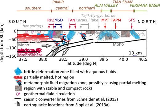
Conceptual lithospheric model along a line from the Southern Pamir to the Fergana Basin, crossing the Pamir Plateau, the Alai Valley, and the Southern Tian Shan Ranges (see Fig. 14). Information on hot and cold regions, occurrence of fluids and melts is mostly derived from the electrical conductivity models (Fig. 15). Solid black lines and arrows resemble seismic converters—suggested lithospheric movements—are taken from Schneider et al. (2013). Undulating arrows mark regions of possible fluid release and migration, triggered by metamorphic reactions (see text).

Special thanks go to the MT field teams, the employees and students of the International Research Center, Russian Academy of Sciences, Bishkek and GFZ Potsdam, Germany: D. Brändlein, X. Chen, A. N. Drokin, T. Krings, L. N. Losihin, E. K. Matiukov, A. A. Nikolaev, A. Nube, P. P. Petrov, M. Schüler, K. Tietze, G. N. Timonin, C. Twardzik and G. Willkommen. From the Tajik side: V. E. Minaev, N. Radjabov, I. Oimahmadov, A. R. Faiziev, all Academy of Sciences of the Republic of Tajikistan, Dushanbe. All colleagues participating in the TIPAGE project contributed with numerous instructive discussions. Many thanks to A. Babeyko, R. Gloaguen, J. Kley, J. Mechie, J. Pfänder, B. Schurr, S. Sobolev, T. Voigt and X. Yuan. Especially the TIPAGE PhD students from Potsdam F. Schneider, S. Schröder and C. Sippl, supplied ideas and support at all stages of the presented work. B. Moldobekov, H. Echtler, A. Mikolaichuk of the Central Asian Institute for Applied Geosciences, Bishkek, and S. K. Negmatullaev, PMP International/Seismic Monitoring Network in Tajikistan, Dushanbe, helped administratively. Most figures were produced using Python and the Matplotlib library (Hunter 2007). We very gratefully acknowledge funding from the DFG (within the bundle project TIPAGE (PAK 443)) and GFZ. Seismic and MT instruments were provided by the GFZ Geophysical Instrument Pool (GIPP). Many thanks to the editor Gary Egbert and two anonymous reviewer for thoughtful comments and suggestions, which helped to improve earlier versions of the manuscript.

REFERENCES