


Abstract
Reconstructions of the Holocene geomagnetic field and how it varies on millennial timescales are important for understanding processes in the core but may also be used to study long-term solar-terrestrial relationships and as relative dating tools for geological and archaeological archives. Here, we present a new family of spherical harmonic geomagnetic field models spanning the past 9000 yr based on magnetic field directions and intensity stored in archaeological artefacts, igneous rocks and sediment records. A new modelling strategy introduces alternative data treatments with a focus on extracting more information from sedimentary data. To reduce the influence of a few individual records all sedimentary data are resampled in 50-yr bins, which also means that more weight is given to archaeomagnetic data during the inversion. The sedimentary declination data are treated as relative values and adjusted iteratively based on prior information. Finally, an alternative way of treating the sediment data chronologies has enabled us to both assess the likely range of age uncertainties, often up to and possibly exceeding 500 yr and adjust the timescale of each record based on comparisons with predictions from a preliminary model. As a result of the data adjustments, power has been shifted from quadrupole and octupole to higher degrees compared with previous Holocene geomagnetic field models. We find evidence for dominantly westward drift of northern high latitude high intensity flux patches at the core mantle boundary for the last 4000 yr. The new models also show intermittent occurrence of reversed flux at the edge of or inside the inner core tangent cylinder, possibly originating from the equator.
1 INTRODUCTION
Global time-varying field models based on direct field measurements spanning the last few centuries (Bloxham et al.1989; Bloxham & Jackson, 1992; Jackson et al.2000) have greatly improved our understanding of the geomagnetic field and how it varies on decadal to centennial timescales, but do not provide a record of sufficient length to understand the physical processes that control the long-term changes in the geodynamo. Such models can be extended to millennial timescales using global compilations of palaeomagnetic field measurements obtained from archaeological artefacts, igneous rocks and lake or marine sediments (Korte et al.2005; Genevey et al.2008; Donadini et al.2009). Over recent years major efforts have been made using these data compilations to reconstruct not only the dipole (Genevey et al.2008; Knudsen et al.2008; Valet et al.2008; Nilsson et al.2010) but also higher order structures of the field (Hongre et al.1998; Constable et al.2000; Korte & Constable 2003; Korte et al.2011; Licht et al.2013).
Such reconstructions can be used in a wide range of applications including investigations of westward and eastward motions in the core (Dumberry & Bloxham 2006; Dumberry & Finlay 2007; Wardinski & Korte 2008), the dynamics of high latitude flux patches (Korte & Holme 2010; Amit et al.2011), field asymmetry related to archaeomagnetic jerks (Gallet et al.2009) and lopsided inner core growth (Olson & Deguen 2012), geomagnetic field shielding of cosmic rays with implications for solar activity reconstructions (Muscheler et al.2007; Snowball & Muscheler 2007; Lifton et al.2008) and as relative dating tools for geological and archaeological archives (Lodge & Holme 2009; Pavón-Carrasco et al.2009; Barletta et al.2010).
Palaeomagnetic data are usually divided into two groups: (i) archaeomagnetic data (here taken to include lavas) containing spot readings in time of both direction and intensity and (ii) sedimentary records constituting continuous depositional sequences of directions and relative intensities. Data from the latter group are generally considered less reliable but provide a better spatial and temporal (ST) geographical distribution, which is essential for global field modelling. Comparisons between dipole moment and dipole tilt reconstructions with more comprehensive spherical harmonic models highlight potential problems with recovering even the most basic (i.e. dipole) component of the field (Knudsen et al.2008; Valet et al.2008; Nilsson et al.2010). One of the main reasons for these differences stems from the use and treatment of sedimentary data to constrain the models. Several studies have noted inconsistencies within the current sedimentary database (Donadini et al.2009), which are mainly due to dating uncertainties (Korte et al.2009; Nilsson et al.2010; Korte & Constable 2011; Licht et al.2013), sometimes on the order of thousands of years (Doner 2003; Nourgaliev et al.2005). In addition to uncertainties related to dating, the magnetic signal may also be both offset in time and inherently smoothed because of the gradual, but largely unknown, process by which the magnetization is locked in to the sediments (see Roberts & Winklhofer 2004). Sedimentary records can also contain systematic errors in both declination and inclination due to problems with orienting the retrieved sediment cores (e.g. Constable & McElhinny 1985; Ali et al.1999; Snowball & Sandgren 2004; Stoner et al.2007) but also due to different problems related to sedimentary processes, such as compaction, which may lead to shallow inclinations (Blow & Hamilton 1978; Anson & Kodama 1987; Tauxe, 2005). A lack of consistent data treatment and/or data availability makes it difficult to estimate these data uncertainties (Panovska et al.2012).
In this study, we present three new palaeomagnetic field models spanning the last 9000 yr (pfm9k), building on the recent work of Korte et al. (2011). One of the main purposes of this study is to address the issues with the sedimentary records mentioned above in order to extract more information from this data set. We do this by introducing new data treatments including redistributions of weight given to the different data sources and types during the inversion and new adjustments/calibrations of relative data based on preliminary field estimates. The results are evaluated by comparisons with other models for the same time period and models based on synthetic data sets derived from the historical field model gufm1 (Jackson et al.2000).
2 DATA
2.1 Initial data set
The palaeomagnetic data used to develop the new models were based on a similar initial data set used to construct CALS10k.1b (Korte et al.2011). This data set consists of archaeomagnetic declination, inclination and intensity data obtained from the online GEOMAGIA50 database (Donadini et al.2006; Korhonen et al.2008) 2013 August 22, and sedimentary palaeomagnetic declination, inclination and relative palaeointensity records from the SED12k data compilation (Donadini et al.2009; Korte et al.2011).
Prior to making any adjustments, the following data, regarded as unsuitable for the modelling procedure, were rejected or replaced based on information in the original publications or comparisons with other data: (i) two lake sediment records, Vatndalsvatn (Thompson & Turner 1985) and Lakes Naroch and Svir (Nourgaliev et al.2005) that were dated using bulk sediment radiocarbon dates that produce suspiciously old ages, were removed. It is a known problem that radiocarbon dating of bulk sediments can produce too old ages due to the incorporation of ‘old’ carbon from the bedrock or soil ‘diluting’ the contemporary 14C in the sediments (see, e.g. Björck & Wohlfarth 2001). In the case of Vatndalsvatn, for example, the offset between calibrated 14C age and true age produced by this effect has been estimated to c. 1200 yr using a combination of lead isotopes, caesium and radiocarbon analyses (Doner 2003). (ii) Likewise all archaeomagnetic data with large dating uncertainties (σage > 500 yr) were also removed. (iii) Two relative palaeointensity records (AAM, WPA—see Table 1 for full names) and one declination record (VIC) were removed based on incompatible long-term trends over the Holocene. If included, most of the data from these records would be removed as outliers anyway during the model rejection analyses (see Section 3.1). (iv) Finally, the relative palaeointensity data from four Scandinavian lake records (FUR, FRG, MOT and SAR), which had been standardized for construction of a Fennoscandian master curve FENNORPIS (Snowball et al.2007), were replaced with the originally published data (Ian Snowball, 2012, personal communication).
2.2 Resampling the sedimentary data
The SED12k data compilation consists of a mix of data from single core studies represented by individual measurements to smoothed data stacks based on multiple measurements from several parallel cores. In addition, the measurements are either performed on discrete samples, collected every 2–3 cm, or on 1–2 m long u-channels samples. The latter usually results in more data points, often with a 1-cm resolution, but each measurement represents an average over a depth range of 15–20 cm depending on the size of the sense-coil and the shape of the pick-up function (Weeks et al.1993). The heterogeneous nature of the data set leads to an inappropriate weighting of the data during the modelling. For example, a u-channel record from a single core (WPA), which consists of correlated measurements, is represented by more than six times as many data points than another arguably more reliable record (BIW) from the same region, based on measurements from three parallel cores, where only the smoothed data are available. To avoid such problems we binned all sedimentary records in 50-yr bins giving equal weight to each site at any given time. This approach reduces the number of sedimentary data by more than 70 per cent (from 67 802 to 19 865), which effectively adds weight to archaeomagnetic data.
2.3 Prior dipole field model
To rescale/adjust the sedimentary palaeomagnetic data and to assign intensity uncertainties we use a prior dipole field model. This model was constructed by combining a dipole tilt reconstruction, DEFNBKE (Nilsson et al.2011), based on selected sedimentary data, with a dipole moment estimate based on cosmogenic radionuclides. Cosmogenic radionuclides (e.g. 10Be, 14C) are produced in the atmosphere by interactions with cosmic rays at a rate which is inversely related to the strength of the geomagnetic field (Lal & Peters 1967). To estimate variations in the dipole moment we used 10Be flux data from the GRIP ice core (Muscheler et al.2004; Vonmoos et al.2006), which were first low-pass filtered with a cut-off frequency of 1/3000 yr−1 to remove solar activity induced production variations (Muscheler et al.2005). The 10Be flux data were then converted to dipole moment using the transfer function from Lal (1988) and normalized by minimizing the resulting dipole field model misfit to all available archaeointensity data (ignoring data uncertainty estimates) over the model time period. The dipole component from gufm1 was added to extend the model to the present, resulting in a gap between 1350 and 1590 AD that was bridged by linear interpolation. See Section 4.2 (Fig. 6) for comparisons between the prior dipole field model and other geomagnetic field models.
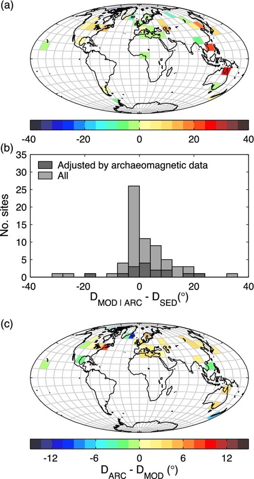
The mean difference between the declination predicted by either regional archaeomagnetic data (DARC) or the dipole prior (DMOD) and the declination from each sediment record (DSED) over overlapping time intervals. Upper panel (a and b) shows the mean difference determined for all records within each grid-cell and lower panel (c) shows the mean difference between adjustments determined using archaeomagnetic data and the dipole prior within each grid, where applicable.
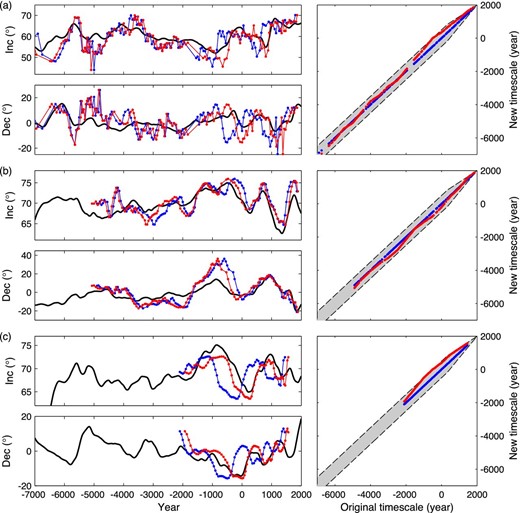
Example of timescale adjustments, shown for (a) Fish Lake, (b) Loch Lomond and (c) Lake Aslikul. For each example the subplots are organized as follows: Inclination (upper left), ceclination (lower left) and timescale (right). Original timescale (blue), adjusted timescale (red) and pfm9k.1 model prediction (black). The light grey shaded area shows the minimum and maximum allowed timescale adjustments.
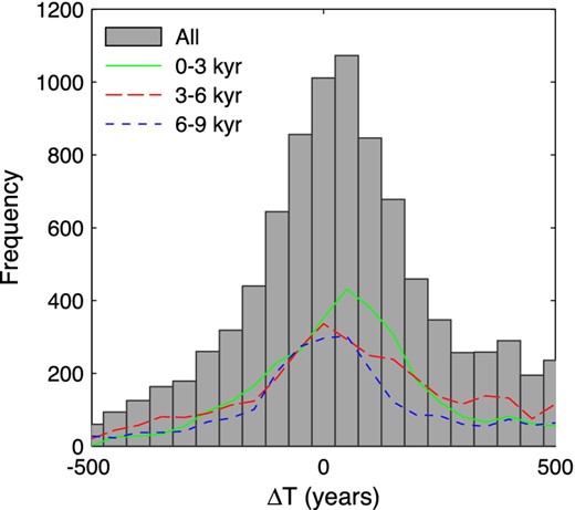
Histogram of all timescale adjustments made to the sedimentary data defined as ΔT = Tadjusted − Toriginal, where T is the age estimate of individual data points. Also shown are the distributions of ΔT for the last 3000 yr (solid green line), between 4000 and 1000 BC (long dashed red line) and between 7000 and 4000 BC (short dashed blue line).
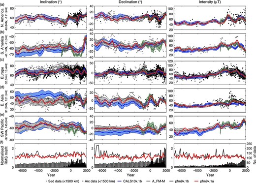
Examples of model predictions of declination (left), inclination (middle) and intensity (right) for five globally distributed locations (a–e) compared to timescale-adjusted sedimentary (grey) and archaeomagnetic data (black) from within a 1500 km, relocated based on an axial dipole. Note that the y-axes have been adjusted to capture the main variations in both model and data and may in some cases exclude extreme values. Bottom panel (f) shows the normalized rms misfits of pfm9k.1a and pfm9k.1b and the data distribution through time of the three different components.
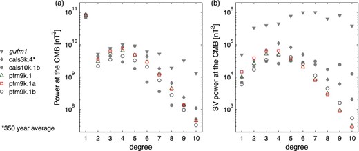
Time-averaged power spectra of (a) main field and (b) secular variation of the three new models (hollow symbols) and a three models shown for reference gufm1 (grey solid symbols). The gauss coefficients of the CALS3k.4 were smoothed with a 350-yr running average prior to calculating the power spectra.
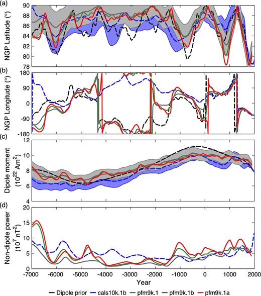
(a) North geomagnetic pole (NGP) latitude, (b) NGP longitude, (c) dipole moment and (d) sum of non-dipole field power of dipole field prior (dashed black line), CALS10k.1b (dashed blue line), pfm9k.1 (green line), pfm9k.1b (grey line) and pfm9k.1a (red line). Uncertainty estimates from the bootstraps of CALS10k.1b (blue) and pfm9k.1b (grey) for NGP latitude and dipole moment are shown as light shaded areas. Note that some of the jumps in the NGP longitude, due to the circularity of the data, have been removed to make the figure clearer. The following sediment records were selected for each location (see Table 1 for full names): (a) FIS, LOU, MAR, (b) CAM, ESC, MNT, TRE, (c) AD1, AD2, ANN, BEG, BOU, EIF, FRG, FUR, GEI, LOM, MEE, MEZ, MOR, MOT, NAU, POH, SAR, SAV, TY1, TY2, WIN, (d) BI2, BIW, ERL, FAN, WPA, (e) BLM, GNO, KEI.
2.4 Calibration of sedimentary declination data
Sediment cores are usually azimuthally unoriented and palaeomagnetic declination data measured on sediments are therefore mostly published as relative values, calculated by removing the average over the whole sequence. While in many cases this approach will lead to reasonable results, there is a risk of introducing systematic errors to the data. The cores could potentially be oriented by fitting the declination data from the top of the sequence to historical field measurements (Constable et al.2000), or alternatively to palaeomagnetic measurements of nearby lava flows correlated in time via tephra layers associated with the same eruption (Verosub et al.1986). However, the sediments from the top of the core or next to tephra layers are often not ideal recorders of the geomagnetic field and therefore such adjustments could be problematic. Another problem is that the data published as relative declination are frequently provided to the database as absolute values (i.e. before removing the long-term average) and may therefore be mistaken for oriented data. To reduce any systematic errors introduced to the database by such type of core reorientations, or lack of reorientations, we adjust each sedimentary declination record by a constant number of degrees based on comparisons with the prior dipole field model or, when appropriate, archaeomagnetic data.
For each record, a first correction was determined as the median difference between the prior dipole model prediction and the data. Archaeomagnetic data were then selected from within a radius of 3000 km from each site and relocated using virtual geomagnetic poles (VGPs). Both the sedimentary and the archaeomagnetic declination data were smoothed with a 200-yr moving window at 100-yr intervals and if there are enough overlapping data points (at least 10), a second correction is determined as the median difference between the smoothed data. The smoothing of the data produces more stable adjustments by restricting the comparison to the more robust long-term variations. To avoid corrections based on spurious data the second correction constant was used only in cases when the archaeomagnetic data provided a better fit to the data than the dipole field model, calculated as the mean of the absolute residuals. The difference between the adjustments predicted by the prior model and the archaeomagnetic data in regions where both could be determined is on average around 3.4° (Fig. 1). A summary of all adjustments can be found in Table 1.
Summary of the sediment records used in this study.
| Abb. | Location | Sample | Nbina | α63b | sFb | ΔDMODc | ΔDARCc | ΔTAVGd | ΔTMAXd | Ref.e |
|---|---|---|---|---|---|---|---|---|---|---|
| type | (°) | (μT) | (°) | (°) | (yr) | (yr) | ||||
| AAM | Alaskan margin, Arctic Sea | U-channel | 112 | 3.5 | – | 14.7 | – | 108 | 400 | 1 |
| AD1 | Adriatic Sea, Italy | U-channel | 122 | 3.5 | 6.2 | – | – | −113 | 450 | 2 |
| AD2 | Adriatic Sea, Italy | U-channel | 79 | 3.5 | 6.5 | – | – | 192 | 500 | 2 |
| ANN | Lac d'Annecy, France | Discrete | 43 | 3.4 | – | 3.0 | (0.1) | −42 | 305 | 3 |
| ARA | Lake Aral, Kazhakstan | Smoothed | 25 | 3.5 | – | 14.7 | (16.2) | −259 | 400 | 4 |
| ASL | Lake Aslikul, Russia | Smoothed | 72 | 3.5 | – | 9.5 | (11.1) | 360 | 500 | 5 |
| BAI | Lake Baikal, Siberia, Russia | Smoothed | 61 | 3.5 | 6.7 | (−6.6) | −2.7 | 283 | 500 | 6 |
| BAM | lake Barombi Mbo, Cameroun | Smoothed | 131 | 3.5 | – | -3.5 | – | −55 | 300 | 7 |
| BAR | Lake Barrine, North Queensland, Australia | Discrete | 169 | 6.7 | 4.9 | 34.4 | (46.5) | 26 | 200 | 8,9 |
| BEA | Beaufort sea, Arctic Ocean | U-channel | 84 | 3.5 | 8.9 | −28.2 | (−33.3) | −4 | 300 | 10 |
| BEG | Lake Begoritis, Greece | Discrete | 106 | 2.5 | – | −1.5 | (0.7) | 35 | 250 | 11 |
| BIR | Birkat Ram, Israel | Discrete | 106 | 4.1 | 6.1 | (−2.0) | −0.9 | −181 | 450 | 12,13 |
| BIW | Lake Biwa, Japan | Smoothed | 185 | 3.5 | – | 8.1 | (9.0) | 33 | 400 | 14 |
| BI2 | Lake Biwa, Japan | Smoothed | 108 | 3.5 | 6.3 | 8.8 | (11.8) | 37 | 500 | 15 |
| BLM | Lake Bullenmerri, Western Victoria, Australia | Smoothed | 83 | 3.5 | – | −3.1 | (3.1) | 27 | 195 | 16 |
| BOU | Lac du Bourget, France | Discrete | 35 | 3.2 | – | −1.9 | (0.5) | 90 | 150 | 3 |
| CAM | Brazo Campanario, Argentina | Smoothed | 137 | 3.5 | – | 0.6 | – | −77 | 300 | 17 |
| CHU | Chukchi Sea, Arctic Ocean | U-channel | 155 | 3.5 | 7.5 | −3.8 | – | −34 | 250 | 10 |
| DES | Dead Sea, Israel | Discrete | 133 | 3.7 | – | −1.4 | (−1.4) | −150 | 500 | 18 |
| EAC | Lake Eacham, North Queensland, Australia | Discrete | 106 | 7.5 | 6.5 | 13.7 | (9.1) | −10 | 150 | 8,9 |
| EIF | Eifel maars, Germany | Smoothed | 185 | 3.1 | – | −0.2 | (2.4) | 194 | 500 | 19 |
| ERH | Erhai Lake, China | Discrete | 109 | 4.5 | – | (−6.2) | −4.6 | 98 | 500 | 20 |
| ERL | Erlongwan Lake, China | Smoothed | 81 | 3.5 | – | 17.5 | (19.2) | −15 | 335 | 21 |
| ESC | Lake Escondido, Argentina | Smoothed | 106 | 3.5 | 6.0 | −2.8 | – | 25 | 300 | 22,23 |
| FAN | Lake Fangshan, China | Smoothed | 114 | 3.6 | – | (1.0) | 4.4 | −139 | 500 | 24 |
| FIN | 2 Finnish Lakes, Finland | Smoothed | 190 | 2.5 | – | −0.4 | (4.0) | −74 | 400 | 25 |
| FIS | Fish Lake, Oregon, USA | Discrete | 145 | 4.1 | – | −2.2 | (−1.9) | 119 | 500 | 26 |
| FRG | Frängsjön, Sweden | Discrete | 161 | 3.8 | 7.9 | −2.1 | (3.2) | −163 | 450 | 27,28 |
| FUR | Furskogstjärnet, Sweden | Discrete | 174 | 4.1 | 8.0 | 2.0 | (3.9) | 207 | 500 | 28,29 |
| GAR | Gardar Drift, North Atlantic | U-channel | 168 | 3.5 | 7.4 | (−14.3) | −19.9 | 159 | 500 | 30 |
| GEI | Llyn Geirionydd, Wales, UK | Smoothed | 128 | 3.5 | – | 1.0 | (2.8) | 80 | 300 | 31 |
| GHI | Cape Ghir, NW Afr. Margin | Discrete | 117 | 4.3 | 6.3 | −0.8 | (2.8) | 361 | 500 | 32 |
| GNO | Lake Gnotuk, Western Victoria, Australia | Discrete | 135 | 4.0 | – | -2.0 | (1.5) | −21 | 300 | 16 |
| GRE | Greenland, North Atlantic | U-channel | 162 | 3.5 | – | 8.0 | (6.5) | 144 | 450 | 33 |
| HUR | Lake Huron, Great Lakes, USA | Discrete | 178 | 4.5 | – | 5.7 | (9.1) | 82 | 500 | 34 |
| ICE | Iceland, North Atlantic | U-channel | 174 | 3.5 | – | −1.1 | (−13.6) | 103 | 300 | 33 |
| JON | Jonian Sea, Italy | U-channel | 58 | 3.5 | – | −4.5 | (−1.2) | 361 | 500 | 2 |
| KEI | Lake Keilambete, Western Victoria, Australia | Discrete | 175 | 3.3 | – | −0.8 | (1.1) | 52 | 200 | 16 |
| KYL | Kylen Lake, Minnesota, USA | Discrete | 60 | 4.2 | – | (15.6) | 17.0 | 218 | 500 | 35 |
| LAM | Lake Lama, Siberia, Russia | Discrete | 182 | 4.4 | – | -9.0 | – | −60 | 500 | 36 |
| LEB | Lake LeBoeuf, USA | Smoothed | 88 | 3.5 | 6.8 | (0.8) | 2.8 | 122 | 300 | 37 |
| LOM | Loch Lomond, Scotland, UK | Smoothed | 122 | 3.5 | – | (−0.8) | −0.1 | −109 | 300 | 38 |
| LOU | Louis Lake, Wyoming, USA | Discrete | 27 | 5.0 | – | 6.4 | (5.5) | 36 | 260 | 39 |
| LSC | Lake St. Croix, Minnesota, USA | Discrete | 152 | 4.0 | 6.9 | −0.3 | (−1.7) | 141 | 500 | 35 |
| MAR | Mara Lake, British Columbia, Canada | Smoothed | 106 | 3.5 | – | 0.5 | (1.8) | −171 | 500 | 40 |
| MEE | Meerfelder Maar, Germany | Discrete | 187 | 5.9 | – | 1.5 | (5.6) | 379 | 500 | 41 |
| MEZ | Lago di Mezzano, Italy | Discrete | 105 | 3.7 | 7.5 | (1.6) | 0.7 | 78 | 300 | 42 |
| MNT | Lago Morenito, Argenitna | Smoothed | 176 | 3.5 | – | 5.1 | – | 37 | 300 | 17 |
| MOR | Lac Morat, Switzerland | Discrete | 35 | 3.2 | – | (3.9) | 4.5 | 97 | 180 | 3 |
| MOT | Mötterudstjärnet, Sweden | Discrete | 163 | 4.1 | 7.8 | −1.8 | (3.3) | 48 | 390 | 28,29 |
| NAU | Nautajärvi, Finland | Discrete | 185 | 4.1 | 8.1 | −6.8 | (−1.7) | −39 | 400 | 28,43 |
| PAD | Palmer Deep, Antarctic Peninsula | U-channel | 165 | 3.6 | 7.3 | -4.3 | – | −7 | 300 | 44 |
| PEP | Lake Pepin, USA | U-channel | 146 | 3.5 | 6.3 | – | – | 49 | 250 | 45 |
| POH | Pohjajärvi, Finland | Discrete | 66 | 3.8 | 9.5 | (0.6) | 9.2 | −80 | 390 | 46 |
| POU | Lake Pounui, North Island, New Zealand | Smoothed | 41 | 3.5 | – | 4.1 | (−3.3) | 12 | 180 | 47 |
| SAG | Saguenay Fjord, Canada | U-channel | 140 | 3.5 | – | (1.1) | 8.7 | 103 | 300 | 48 |
| SAN | Hoya de San Nicolas, Mexico | Smoothed | 113 | 3.5 | – | 3.7 | (1.2) | 6 | 100 | 49 |
| SAR | Sarsjön, Sweden | Discrete | 155 | 3.9 | 8.0 | (−0.1) | 2.0 | −108 | 435 | 27,28 |
| SAV | Savijärvi, Finland | Discrete | 122 | 4.5 | – | (-4.0) | 1.6 | −232 | 500 | 28,50 |
| SCL | Lake Shuangchiling, China | U-channel | 166 | 3.8 | – | (26.4) | 24.0 | −24 | 500 | 51 |
| STL | St. Lawrence Est., Canada | U-channel | 150 | 3.5 | 6.6 | 19.0 | (26.8) | −143 | 500 | 52 |
| SUP | Lake Superior, Great Lakes, USA | Smoothed | 184 | 3.6 | – | 4.0 | (8.3) | −105 | 400 | 53 |
| TRE | Laguna el Trebol, Argentina | Smoothed | 141 | 3.5 | 5.8 | 7.9 | – | 18 | 240 | 54,55 |
| TRI | Lake Trikhonis, Greece | Discrete | 133 | 2.9 | – | −2.4 | (1.4) | 243 | 500 | 11 |
| TUR | Lake Turkana, Kenia | Discrete | 51 | 4.1 | – | – | – | −131 | 400 | 56 |
| TY1 | Tyrrhenian Sea, Italy | U-channel | 61 | 3.5 | – | −0.6 | (−1.5) | 119 | 500 | 2 |
| TY2 | Tyrrhenian Sea, Italy | U-channel | 79 | 3.5 | – | −0.5 | (0.5) | 190 | 450 | 2 |
| VIC | Lake Victoria, Uganda | Smoothed | 143 | 3.5 | – | – | – | −10 | 150 | 57 |
| VOL | Lake Volvi, Greece | Discrete | 50 | 2.9 | – | −1.9 | (1.5) | 265 | 500 | 11 |
| VUK | Vukonjärvi, Finland | Discrete | 102 | 4.1 | – | −25.2 | (−15.5) | 225 | 500 | 58 |
| WA1 | PS69/274–1, West Amundsen Sea | Discrete | 16 | – | 9.3 | – | – | 41 | 385 | 59 |
| WA2 | PS69/275–1, West Amundsen Sea | Discrete | 18 | – | 9.1 | – | – | 316 | 500 | 59 |
| WA3 | VC424, West Amundsen Sea | Discrete | 27 | – | 8.8 | – | – | 104 | 400 | 59 |
| WAI | Lake Waiau, Hawaii, USA | Smoothed | 109 | 3.5 | – | −3.1 | (−3.4) | −45 | 385 | 60 |
| WIN | Lake Windermere, Northern England, UK | Smoothed | 137 | 3.5 | – | −3.9 | (−2.5) | 296 | 500 | 31 |
| WPA | West Pacific, West Pacific | U-channel | 187 | 3.5 | – | – | – | 185 | 450 | 61 |
aNumber of bins after resampling.
bMean α63 and sF of binned data used for modeling.
cDeclination adjustment (ΔD) based on prior dipole field model (MOD) or archaeomagnetic data (ARC). Adjustments not used are shown in brackets.
dAverage and maximum timescale adjustments (ΔT), see Section 3.2.
e1, Lisé-Pronovost et al. (2009); 2, Vigliotti (2006); 3, Hogg (1978); 4, Nourgaliev et al. (2003); 5, Nurgaliev et al. (1996); 6, Peck et al. (1996); 7, Thouveny & Williamson (1988); 8, Constable & McElhinny (1985); 9, Constable (1985); 10, Barletta et al. (2008); 11, Creer et al. (1981); 12, Frank et al. (2002b); 13, Frank et al. (2003); 14, Ali et al. (1999); 15, Hayashida et al. (2007); 16, Barton & McElhinny (1981); 17, Creer et al. (1983), 18, Frank et al. (2007); 19, Stockhausen (1998); 20, Hyodo et al. (1999); 21, Frank (Frank 2007); 22, Gogorza et al. (2002); 23, Gogorza et al. (2004); 25, Haltia-Hovi et al. (2010); 26, Verosub et al. (1986); 27, Snowball & Sandgren (2002); 28, Snowball et al. (2007); 29, Zillén (2003); 30, Channell et al. (1997); 31, Turner & Thompson (1981); 32, Bleil & Dillon (2008); 33, Stoner et al. (2007); 34, Mothersill (1981); 35, Lund & Banerjee (1985); 36, Frank et al. (2002a); 37, King (1983); 38, Turner & Thompson (1979); 39, Geiss et al. (2007); 40, Turner (1987); 41, Brown (1981); 42, U. Frank pres. comm.; 43, Ojala & Saarinen (2002); 44, Brachfeld et al. (2000); 45, Brachfeld & Banerjee (2000); 46, Saarinen (1998); 47, Turner & Lillis (1994); 48, St-Onge et al. (2004); 49, Chaparro et al. (2008); 50, Ojala & Tiljander (2003); 51, Yang et al. (2009); 52, St-Onge et al. (St-Onge et al.2003); 53, Mothersill (1979); 54, Gogorza et al. (2006); 55, Irurzun et al. (2006); 56, Barton & Torgersen (1988); 57, Mothersill (1996); 58, Huttunen & Stober (1980); 59, (Hillenbrand et al.2010); 60, Peng & King (1992); 61, Richter et al. (2006.)
The choice of a suitable radius for the selection of archaeomagnetic data is a trade-off between obtaining enough data used to calculate the adjustment while limiting the selection to an area with similar geomagnetic field history. A 3000 km radius can be considered quite large, however; given the Earth's ∼40 000 km circumference, the corresponding 6000 km wavelength translates to spherical harmonic degree 6–7, which is roughly the spatial resolution of our final models (see Fig. 5). We found that the corrections calculated based on a smaller radius often lead to regionally inconsistent adjustments, mainly because of an over-reliance on individual archaeomagnetic data points. The declination adjustments based on a 3000 km radius produce a regionally consistent data set, which differ slightly but systematically from the predictions of the prior dipole field model (Fig. 1c).
2.5 Scaling of relative palaeointensity
The sedimentary relative palaeointensity data were converted to absolute palaeointensites, following the approach of Korte & Constable (2006) and Donadini et al. (2009), by multiplying each entire record with a constant scaling factor. As for the declination data, the scaling factor was calculated based on the prior dipole field model or using archaeomagnetic intensity data, where possible. The scaling factor was determined as the median ratio of the reference palaeointensity data over the relative palaeointensity data.
For each record, a first scaling factor was determined based on the prior dipole field model. The archaeomagnetic data were selected using the same criteria as for the declination adjustments and smoothed using the same 200-yr moving window and used to calculate a second scaling factor. As for the declination corrections the second scaling factor was only used when the archaeomagnetic data provided a better fit to the data than the prior dipole field model, calculated as the mean of the absolute residuals. The scaling factors calculated based on the prior dipole model did not differ considerably (on average 4.5 per cent) from those based on archaeomagnetic data.
Relative palaeointensity reconstructions can be sensitive to changes in the depositional environment through time and such changes could lead to different scaling factors being appropriate for different parts of the sequence. In two cases (LSC at 600 BC and TRE at 0 AD), we found sudden jumps in the data that we identified as such changes in the depositional environment. In both cases suspiciously large changes in the relative palaeointensity could also be traced back to similar changes in concentration dependent mineral magnetic parameters at corresponding depths in the original studies (Lund & Banerjee 1985; Gogorza et al.2006). To avoid applying inappropriate scaling factors both records were split into two parts, which were rescaled separately and then joined back together. We suspect that other relative palaeointensity records may suffer from similar problems, potentially with more gradual changes making them more difficult to identify. Improvements in both the identification and correction of this problem should be investigated in future studies.
2.6 Assigning error estimates
In this study, we acknowledge that the published error estimates may fail to account for unknown systematic errors and have therefore opted for an approach similar to that of Donadini et al. (2009) using a set of minimum error estimates. However, to penalize data with less well-defined uncertainties, different minimum errors were assigned depending on the number of samples/specimens (N/n) used to calculate the mean direction or intensity.
The sedimentary directional data consist of discrete sample measurements (31 records), different forms of running averages (25 records) and u-channel measurements (17 records). The data, especially from the second group, are sometimes published with some form of uncertainty estimate. However, out of all these records only 10 are provided with an error estimates in the database. These come in the form of α95 confidence limits (2), (angular) standard deviations (4) and maximum angular deviations (4). In order to treat the data consistently only the first were deemed suitable for the modelling purposes. These α95 confidence limits are based on stacks of 12 (EIF) and 8 (FIN) parallel cores with equivalent α63 rms values of 3.05° and 1.88°, respectively. While these errors may not be representative of all sedimentary data, the latter study (Haltia-Hovi et al.2010) in particular highlights the potential precision with which the directions can be acquired given enough data. Based on the assumption that most hidden or systematic errors associated with sedimentary data are due to chronologic uncertainties, which are dealt with separately in Section 3.2, and problems with core orientation, partly solved by the declination adjustments, we treat error estimates in a similar way to the archaeomagnetic errors.
For the purpose of error assignment the sedimentary data can be divided into two groups: (i) records containing independent data from discrete samples and (ii) smoothed records (including u-channels) containing non-independent data. From the resampling of the data we obtain uncertainty estimates for both directions and rescaled intensities based on the dispersion of the data within each 50-yr bin. For data from the first group, with no prior error estimates, the resulting uncertainty estimates are treated in the same way as the archaeomagnetic data using the same minimum α63 and sF assigned based on the number of samples used to calculate the mean values. For the data from the second group information is missing regarding both the number of independent data points and the true dispersion of the data. The provided α95 estimates from EIF and FIN were converted to α63 and transferred to binned error estimates through error propagation. Data from these two records were then assigned a minimum α63 = 2.5° while the uncertainty estimates, calculated from the binned data, from the remaining records were treated as less well defined and assigned a minimum α63 = 3.5°. None of the rescaled intensity error estimates from the second group provided in the database were deemed suitable and therefore all uncertainty estimates, calculated from the binned data, were assigned a minimum sF = 12 per cent. The strategy used here to assign uncertainties to sedimentary data results in larger errors on average for both directions (3.8°) and intensities (7.1 μT) compared to the minimum values of 3.5° and 5 μT assigned by Donadini et al. (2009). However the methodology also allows for slightly smaller error estimates: 10 per cent of the α63 are smaller than 3.5° and 11.5 per cent of the sF are lower than 5 μT. The average α63 and sF from each record are listed in Table 1.
3 MODELLING METHOD
3.1 Initial model
The damping parameters for the preferred model were chosen by visual comparison (Lodge & Holme 2009) of the time-averaged geomagnetic power spectra of the main field and secular variation to those of the historical field model gufm1 and the high resolution palaeomagnetic field model CALS3k.4 (Korte & Constable 2011), respectively. The chosen regularization norms result in relatively stronger damping of power in main field and secular variation for higher spherical harmonic degrees (i.e. small-scale/short-term structure) compared to lower spherical harmonic degrees. We assume that a reasonable solution does not show more spatial complexity on average than the historical field and λS is chosen using the average main field power spectra of gufm1 as a template. We attempt to preserve, or avoid exceeding, the relative proportions of the power spectra by limiting the ‘allowed’ power in each spherical harmonic degree based on the power of lower spherical harmonic degrees, according to the gufm1 power spectrum. Given the large dating uncertainties associated with the palaeomagnetic data, we also assume that a reasonable solution will not be able to capture variations on timescales shorter than 300–400 yr. To produce a suitable template for the secular variation power spectra based on this criterion we filter the CALS3k.4 gauss coefficients with a 350-yr running average and λT is chosen by comparison to the average secular variation power spectrum of this temporally smoothed version of the CALS3k.4 model.
The last two steps were repeated. After the first iteration 6.5 per cent of the declination data were rejected (cutoff = 11.15°), 6.4 per cent of the inclination data (cutoff = 10.62°) and 5.1 per cent of the intensity data (cutoff = 37.50 per cent). The absolute change in the declination and relative palaeointensity calibration factors after the first iteration were on average 1.9° and 2.9 per cent, respectively, with changes up to 8° (mainly high latitude sites) and 10 per cent required for some records. After the third iteration less than 0.2 per cent of the data were rejected and changes to the calibration factors were reduced to on average 0.2° and 0.3 per cent. The final model pfm9k.1 was chosen as model B3. To minimize end effects associated with the B-spline functions the model is determined for the period between 7500 BC and 2000 AD but we only show results from 7000 BC to 1900 AD. We decided to keep a relatively larger part of the recent end of the model in order to be able to validate the model against gufm1, even though this part of the model will include some spline end effects.
Regularized models will tend to underestimate, rather than overestimate, the intensity with respect to the data. This is true even if we exclude the dipole coefficients from the regularization, as can be seen in Table 2. The problem can be exacerbated by the inclusion of sedimentary relative palaeointensity records, particularly if they are rescaled using a model that is already underestimating the intensity. Including iteratively rescaled sedimentary data in the residual analysis may also produce near evenly distributed intensity residuals hiding the fact that the model is underestimating the absolute intensity data. This is partly resolved by resampling the sedimentary data, effectively increasing the weight of the archaeomagnetic, absolute, intensity data. To further improve the fit we also increased the weight given to all intensity data by 50 per cent, which was achieved by reducing the uncertainty estimates of the data accordingly during the inversion process. A similar approach was used by Korte & Constable (2005), but with a 100 per cent increase in the weight. We found that a 50 per cent increase provided a good balance between improving the model fit to the intensity data, reducing the model underestimation, while not markedly changing the overall rms misfit to the data (including directions).
Model-data residuals, archaeomagnetic data.
| Modela | NARCb | FAVGc | rmsFd | rmsARCd |
|---|---|---|---|---|
| ARCH3k.1 | 10110 | 1.09 | 1.46 | 1.57 |
| CALS10k.1b | 12043 | 3.23 | 1.77 | 1.88 |
| Dipole field prior | 12043 | −0.15 | 1.72 | 2.19 |
| pfm9k.0 (initial) | 12043 | 2.97 | 1.78 | 1.81 |
| pfm9k.0 (dec. data adjusted) | 12043 | 2.48 | 1.75 | 1.79 |
| pfm9k.0 (sed. data resampled) | 12043 | 1.16 | 1.64 | 1.69 |
| pfm9k.1 (increase weight to F) | 12043 | 0.66 | 1.58 | 1.69 |
| pfm9k.1a (sed. timescales adjusted) | 12043 | 0.72 | 1.58 | 1.68 |
aDifferent pfm9k models listed with more data treatments (in brackets) added successively from top to bottom.
bNumber of archaeomagnetic data (dec + inc + F) between −7000 and 1900 AD used for the residual analyses.
cAverage intensity residuals.
dThe rms of residuals for intensity and all data, normalized by their individual uncertainty estimates.
3.2 Addressing sediment age uncertainties
The age uncertainties of the data are often not well constrained and therefore applying a strong temporal damping seems a reasonable approach. This will be effective if the age uncertainties can be considered to be non-systematic, for example for the archaeomagnetic data where most data points have been dated individually. However, for the sedimentary data the age estimates can be both systematically wrong, for example due to reservoir effects affecting the radiocarbon dates, and have correlated errors due to the interpolation of ages when constructing an age depth model. Given the stratigraphic information of the data we can attempt to correct for this by finding an optimal age-depth model for each sedimentary record based on comparisons to a preliminary model prediction (Fig. 2). In regions where the model is not overly dependent on individual records this approach should be able to correct for inconsistencies in the data set that are due to incompatible age-depth models. In contrast, in regions where data are scarce this approach will result in few or no adjustments to the timescales. For this analysis we used the initial data set (before outlier rejection) and the pfm9k.1 model.
In Fig. 2, we show examples from three different records of data plotted against their original timescales and the optimally adjusted timescales compared with predictions of the pfm9k.1 model. All three records show time adjustments of 300 yr or more, both towards younger and older ages. The top 4000 yr from the Fish Lake record (FIS) has been shifted on average 288 yr towards younger ages. This is supported by a similar adjustment of ∼280 yr which was suggested by Hagstrum & Champion (2002), due to calcium carbonate dilution of the bulk 14C samples used to date the record. The Fish Lake chronology was also forced to fit an independent age estimate of the Mazama Tephra layer, of about 4800 BC (Verosub et al.1986), which explains why the model predicts only minor time adjustments for this older part of the record. Fig. 3 shows the distribution of timescale adjustments defined as ΔT = Tadjusted − Toriginal, where T is the age estimate of individual data points. Overall the distribution is slightly skewed towards younger ages, particularly for the last 3000 yr where the model is more heavily constrained by archaeomagnetic data. This could suggest either a widespread ‘old’ carbon problem affecting the radiocarbon based chronologies or possibly a predominant lock-in delay effect.
3.3 Addressing all data uncertainties
To investigate the effects of magnetic and age (MA) uncertainties as well as the impact of the ST distribution of the data we used the MAST bootstrap methodology, described in detail in Korte et al. (2009). First a temporary model pfm9k.1B was constructed based on the same approach as above but with a more relaxed temporal damping, chosen by visual comparison to the secular variation power spectra of gufm1. For each of the 2000 bootstrap samples we created data sets by drawing on the final pfm9k.1B data set. The bootstrap models were constructed without further iterative recalibration or rejection of data and using the same damping parameters as for pfm9k.1B. The simulated data at each location were generated in two steps with slight differences for archaeomagnetic and sedimentary data. (i) In the first step the archaeomagnetic data were independently sampled from two normal distributions, one centred on the value of the magnetic component with a standard deviation corresponding to the data uncertainty estimate, and the other centred on the age estimate and using its respective standard error. For the sedimentary data the sampling of each datum from a normal distribution centred on the magnetic component was done in the same way. However, for the temporal sampling the timescale of each record was instead randomly stretched and compressed using the same routine described above. This introduces rather large, but from what we can infer from the analysis in Section 3.2 also quite realistic, chronological errors that increase with age. (ii) In the second step, bootstraps were performed on these data sets, where for the archaeomagnetic data the number of data locations was kept constant and values picked by uniform random sampling from that data set. For the sediments, the number of records was kept fixed and the locations again uniformly sampled. The final model, pfm9k.1b, was based on the average of the 2000 bootstrap models and the uncertainties determined as standard deviation of the coefficients. The number of 2000 models was found to be enough to reach convergence.
4 MODEL RESULTS AND COMPARISONS
We have constructed three new models of the geomagnetic field variation for the last 9000 yr; (i) pfm9k.1 based on the initial data set with strong temporal damping, (ii) pfm9k.1a based on an optimally timescale-adjusted data set with strong temporal damping and (iii) pfm9k.1b: the average of 2000 bootstrap models with weak temporal damping.
4.1 Model-data comparisons
By reducing inconsistencies in the sedimentary age estimates, pfm9k.1a is able to capture larger amplitude palaeosecular variation (PSV) than other models that include sedimentary data, such as pfm9k.1b and CALS10k.1b (Fig. 4). The predictions of pfm9k.1a are in good agreement with models based on archaeomagnetic data, for example A_FM (Licht et al.2013), ARCH3k.1 (Korte et al.2009), for the northern hemisphere sites where the latter models can be considered more robust. Well known PSV features such as the westward declination swing in Europe around 700 BC, between declination features ‘f’ and ‘e’ originally labelled by Turner & Thompson (1981), and the steep rise in inclination in North America around the same time tend be smoothed out in models that incorporate sedimentary data. This is mainly due to the often relatively large (up to 500 yr) inconsistencies between age estimates for sediment records from the same regions. We also note that in regions where the field is less well constrained, for example South America, the sediment timescale adjustments could potentially also amplify noise present in the pfm9k.1 model.
Resampling the sedimentary data has reduced the influence of data from a few overrepresented records and also given more weight to archaeomagnetic data. This is particularly noticeable in East Asia and South America where CALS10k.1b appears to be heavily dependent on two u-channel records (WPA and PAD). The strong influence of these two records in CALS10k.1b leads to an underestimation of intensity in East Asia for the last 2000 yr and causes a general underfitting to other data from the same region, seen in all three components (Fig. 4).
The effects of the declination adjustments are most obvious in East Asia and the SW Pacific where our new models, based on the adjusted data, do not show a similar persistent westward offset as predicted by CALS10k.1b (Fig. 4). As shown in Fig. 1 and Table 1, several declination records from both SW Pacific and East Asia required adjustments of more than 10° in the same direction (BAR, EAC, ERL and SCL). All of these corrections were based on comparisons to archaeomagnetic data, which would suggest that this systematic offset seen in the sedimentary declinations from this region is not a real feature of the geomagnetic field. On the other hand, the archaeomagnetic data from the SW Pacific are both few and scattered, as shown in Fig. 3, and we acknowledge that the declination adjustments applied to the data from this region are rather uncertain.
Time variation of the rms model-data residuals normalized by the data uncertainties for pfm9k.1a and pfm9k.1b are shown in Fig. 4 and a summary for all three models is provided in Table 3. The misfits are calculated on the respective outlier free data sets and therefore differ slightly from the values obtained in Table 2. Due to the relaxed temporal damping the outlier free data set of pfm9k.1b contains slightly more data than the pfm9k.1 data set and due to the adjustments of the sedimentary record timescales even fewer outliers are removed in the final pfm9k.1a data set. The pfm9k.1b model has considerably higher rms misfits than both pfm9k.1 and pfm9k.1a owing to the increased temporal smoothness. Not surprisingly the pfm9k.1a model has the smallest rms misfit of all models with the main improvements seen in the fit to the sedimentary data.
Model-data rms, final data sets.
| Model | NALLa | RMSDECb | RMSINCb | RMSFb | RMSARCb | RMSSEDb | RMSALLb |
|---|---|---|---|---|---|---|---|
| pfm9k.1 | 29051 | 1.15 | 1.27 | 1.14 | 1.27 | 1.16 | 1.20 |
| pfm9k.1a | 29422 | 1.09 | 1.23 | 1.12 | 1.26 | 1.08 | 1.16 |
| pfm9k.1b | 29207 | 1.26 | 1.36 | 1.21 | 1.34 | 1.26 | 1.30 |
| Model | NALLa | RMSDECb | RMSINCb | RMSFb | RMSARCb | RMSSEDb | RMSALLb |
|---|---|---|---|---|---|---|---|
| pfm9k.1 | 29051 | 1.15 | 1.27 | 1.14 | 1.27 | 1.16 | 1.20 |
| pfm9k.1a | 29422 | 1.09 | 1.23 | 1.12 | 1.26 | 1.08 | 1.16 |
| pfm9k.1b | 29207 | 1.26 | 1.36 | 1.21 | 1.34 | 1.26 | 1.30 |
aNumber of data (dec+inc+F) between −7000 and 1900 AD used for the residual analyses.
bThe rms of residuals for different data types and sources, normalized by their individual uncertainty estimates.
4.2 Dipole versus non-dipole field
The comparison of time-averaged main field power spectra in Fig. 5 reveals that all new models have less power in the quadrupole terms than both gufm1 and CALS10k.1b (Fig. 5). In the case of CALS10k.1b this is mainly due to differences in |$g_2^0$| and |$g_2^2$|, which in turn appear to be related to the resampling of the sedimentary data and the declination adjustments. Due to the way we choose the damping parameters, attempting to preserve the relative proportions of the time-averaged gufm1 power spectra, the new models also show similarly suppressed power in all higher degree terms. Based on end-to-end simulations using synthetic data sets Licht et al. (2013) found a general tendency of the models to underestimate the |$g_2^1$| component. If the same applies to our new models, it could suggest that the observed low power in the quadrupole, relative to gufm1, is due to a bias in the data set. On the other hand, it is also possible that the power spectrum of the historical field is not representative of the field on longer timescales. In either case the power in the higher degree terms (l > 2) of the new models may have been excessively suppressed.
The time-averaged secular variation spectra of all three models are fairly similar to each other, with pfm9k.1b exhibiting slightly less power and pfm9k.1a slightly more power in degrees 1–4. The resulting temporal resolution of the models is estimated to 300–400 yr by comparing the power spectra of model predictions (declination, inclination and intensity) at different coordinates.
The dipole field variation, that is the movement of the north geomagnetic pole (NGP) and changes in dipole moment, of all three new models are fairly similar (Fig. 6). The largest variation is seen in pfm9k.1a but it rarely strays outside the pfm9k.1b one sigma confidence limit. Apart from a slight decrease in NGP colatitude around 1800 AD, all new models show quite good reproducibility with NGP positions of the prior dipole field model for the last 400 yr (based on gufm1). The NGP movements of the new models are also in good agreement with the dipole field model for the earlier parts (based on DEFNBKE), although mostly with slightly lower co-latitudes. The NGP longitude of the new models and CALS10k.1b diverge slightly between 4000 BC and 1500 AD, but in general the models agree well and the differences are within the uncertainty limits. All reconstructions, but particularly pfm9k.1a and the dipole field prior, suggests the presence of a 2700- or 1350-yr periodicity signal in the dipole tilt variation previously noted by both Nilsson et al. (2011) and Korte et al. (2011).
In common with the prior dipole field model and CALS10k.1b the new models predict relatively low dipole moments around 6000 to 4000 BC increasing and reaching a maximum around 1000 BC to 1000 AD (Fig. 6c). The new models predict on average higher dipole moments than CALS10k.1b for the earlier part of the record, where the models are more dependent on sedimentary data, but mostly agree within the uncertainty estimates. The dipole moments of the new models are also high when compared to prior dipole field model for the last 400 yr (based on gufm1), but predict roughly the same negative slope. By successively excluding different data types we found that this potential overestimation of the dipole moment for the recent end of the model is related to the introduction of sedimentary directional data. It is possible that the declination adjustment of a few records based on the dipole prior model may have forced the field to become more dipolar, however, this needs to be investigated further.
Fig. 6(d) shows the power of the sum of all the higher-degree, non-dipole, harmonics of the different models compared through time. The most striking feature is the relatively low non-dipolar field predicted by the new models between 4000 and 1500 BC. This coincides with the period where the NGP longitude deviates slightly from CALS10k.1b and is related to the adjustments made to the sedimentary data. Such low non-dipolar field appear unrealistic and indicates that the models may not be well constrained during this period in time.
4.3 Radial field at the core-mantle boundary
In Fig. 7, we compare time-averages/time-slices of Br at the CMB for pfm9k.1a, pfm9k.1b and the most recent global models for three different time-periods. The structures shown by the new models and CALS10k.1b are similar for the long-term time-average, 7000 BC to 1900 AD (Fig. 7a). All three models show two high latitude areas that preferentially exhibit high intensity flux in the southern hemisphere, beneath South America and the Pacific Ocean, although the latter feature is slightly less pronounced in pfm9k.1b. In addition, both pfm9k.1a and pfm9k.1b show indications of two persistent high latitude high intensity flux patches in northern hemisphere, beneath Greenland and Western Russia. The northern and southern hemisphere high latitude flux patches are not symmetrically located around the equator. However, due to the poor data coverage for the southern hemisphere, the location of these flux patches are more uncertain. As pointed out by Licht et al. (2013), and as we will see in Section 5, there is a risk that the occurrence of these features is related to a sampling bias. The new model shows a less pronounced SW pacific anomaly compared to CALS10k.1b due to the declination adjustments and the resampling of the sedimentary data. The persistent anomaly also has a different signature compared to CALS10k.1b, characterized by comparatively weaker flux beneath the Fiji islands.
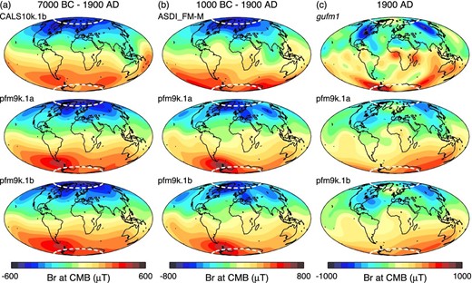
(Upper panel) Time-averaged radial component of the field (Br) at the core mantle boundary (CMB) predicted by representative models for each time period: (a) CALS10k.1b 7000 BC to 1900 AD, (b) ASDI_FM 1000 BC to 1900 AD and (c) gufm1 1900 AD. Br predictions over the same time periods for pfm9k.1a (middle panel) and pfm9k.1b (lower panel). The dashed white lines show the CMB expression (∼71° N/S) of the inner core tangent cylinder.
The new models time-averaged Br for the last 3000 yr is characterized by more variable field structure in the northern hemisphere compared to the longer time average (Fig. 7b). There are three areas that preferentially exhibit high intensity fluxes beneath Greenland, Europe and Eastern Asia. Both pfm9k.1a and pfm9k.1b also exhibit generally more complex structure at high latitudes in the northern hemisphere compared to the recently published ASDI_FM-M model (Licht et al.2013). The SW Pacific anomaly is again not as pronounced in the new models compared to both in CALS10k.1b and ASDI_FM-M, due to the above-mentioned adjustments of the sedimentary data. Instead the new models predict a persistent strong flux beneath East Asia.
Fig. 7(c) shows the Br prediction at the CMB of the two models for the year 1900 AD compared to the prediction of gufm1. The northern hemisphere predictions of both models are relative accurate but smoothed, roughly equivalent to the gufm1 model prediction truncated at spherical harmonic degree 5–6 (see Fig. 8). The southern hemisphere reconstruction, on the other hand, provides much less higher order structure and is dominated by spherical harmonic degree 3–4. The two southern hemisphere high latitude high intensity flux patches present in gufm1 are represented as one diffuse area of high flux in pfm9k.1a. The comparison provides a direct, although slightly limited, evaluation of how much structure we can expect the models to capture. We note that sedimentary palaeomagnetic data, which are particularly important for the southern hemisphere reconstruction, are poorly represented in the last few centuries of the database, mainly due to the difficulty in getting a reliable signal from the top sloppy part of sediment cores.
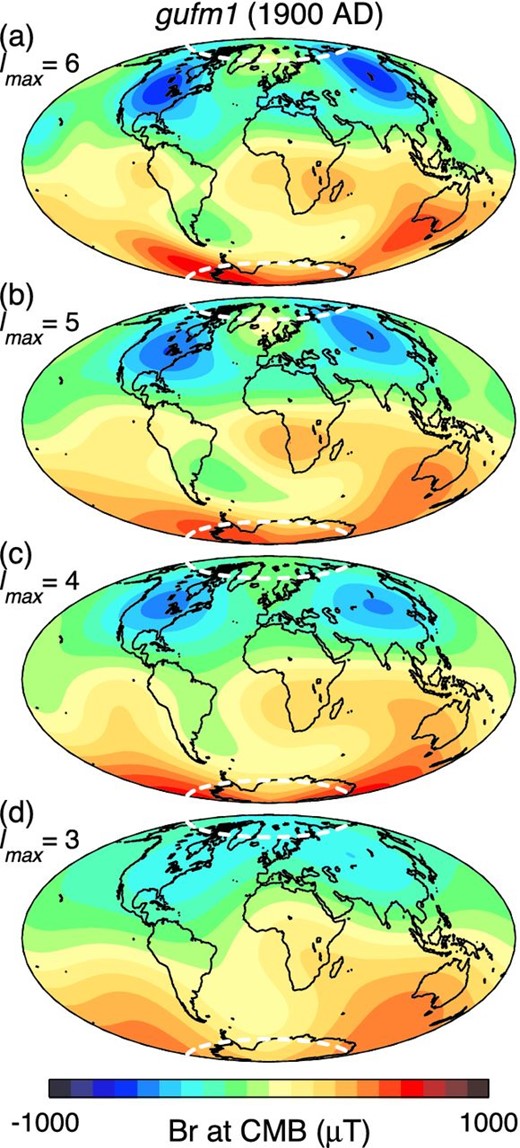
Comparison of the radial component of the field (Br) at the core mantle boundary (CMB) predicted by gufm1 truncated at (a) degree lmax = 6, (b) degree lmax = 5, (c) degree lmax = 4 and (d) degree lmax = 3. The dashed white lines show the CMB expression (∼71° N/S) of the inner core tangent cylinder.
Fig. 9 shows five different time slices of the pfm9k.1a Br at the CMB. We focus on the last 4000 yr where the model is best constrained. For a more complete illustration the reader is referred to the animations provided with the Supporting Information (mov1–3). Throughout the selected time period the southern hemisphere Br prediction is characterized by the appearance and disappearance of two high latitude high intensity flux patches beneath South America and the SW Pacific. There is not much movement between them and for the most part they are situated at the edge of the tangent cylinder. The Br prediction for the northern hemisphere reveals a much more dynamic behaviour. The northern hemisphere structure is dominated by the presence of two, but sometimes three, high latitude high intensity flux patches which move with an overall westward motion around the edge of the tangent cylinder. The movement or disappearance/emergence of flux patches is heavily smoothed due to the strong temporal damping but appears to describe a stop-and-go motion with an average rate equivalent to a 5000-yr rotation period. The apparent westward high latitude flux motion correlates well with a more or less continuous westward movement of the NGP between −1800 and 600 AD (Fig. 6). The NGP then moves eastwards up to about 500 AD during which the high latitude flux motion breaks down and the field structure becomes more complex.
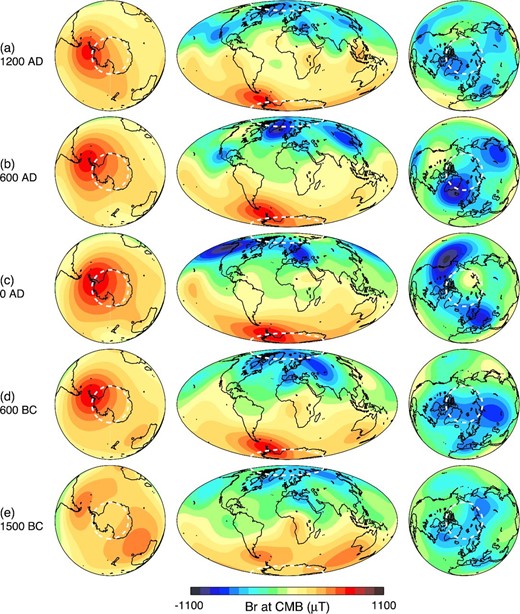
Radial component of the field (Br) at the core mantle boundary (CMB) of pfm9k.1a at (a) 1200 AD, (b) 600 AD, (c) 0 AD, (d) 600 BC and (e) 1500 BC. Southern hemisphere (left) and northern hemisphere (right) orthographic projections added for clarity. The dashed white lines show the CMB expression (∼71° N/S) of the inner core tangent cylinder.
The field evolution at the CMB predicted by pfm9k.1a, in particular, also shows a recurrence of reversed (or weak) flux just at the edge of the tangent cylinder in the northern hemisphere around −1500, −300, 700 and 1900 AD. These reversed flux patches appear in association with, and at the far side of, two high latitude high intensity flux patches predominantly situated in one hemisphere. In at least two cases (−300 and 1900 AD) they seem to originate from the equator and move northwards towards the edge and possibly into the tangent cylinder over a period of a few centuries. However, due to the truncation level of the models it may not be possible to track any movement into the tangent cylinder (see comparison with gufm1 at different truncation levels, Figs 7–8).
5 EVALUATION OF MODELS USING GUFM1
To investigate how well we can expect our models to resolve the field structure at the CMB we generated a set of synthetic data sets with the same data uncertainties and the same ST data distribution as the final outlier free pfm9k.1 data set. The synthetic data sets were resampled in time and space from a reasonably realistic field description, a reference field model, covering the investigated time interval. MA data uncertainties were added in the same way as for the construction of pfm9k.1b, but with the distinction that the data age estimates were kept constant and age uncertainties were introduced to obtain the reference field model predictions. Finally, a new set of synthetic models was produced based on the synthetic data sets and the same damping parameters as for the final pfm9k.1 model. The model performance was evaluated by comparing the Br at the CMB of the synthetic model and the reference field model.
The choice of a suitable reference field model is important and will to some degree influence the results. For a similar type of analysis Licht et al. (2013) used a periodically extended version of the gufm1 model, covering the last three millennia. Here, we have instead opted to use single time-slices, also derived from the gufm1 model, extended back in time by adding a continuous 5000-yr westward rotation to the whole field. The advantage of this approach is that it provides a direct test of the robustness of the observed westward drift pattern observed in the palaeofield models. An initial reference field model was constructed using the gufm1 prediction at 1840 AD and extended backwards and forwards in time with a continuous westward rotation to cover the palaeofield model time period −7000 to 1900 AD. An animation showing the time variation of the Br at the CMB for this reference field model and the corresponding synthetic model is provided in the Supporting Information (mov4).
Because of the nature of the regularization, to minimize field structure at the CMB, the model performance test will be more sensitive in areas where the reference field model shows more structure, for example in the vicinity of high intensity flux patches. To reduce the impact of such ST differences in a particular reference field model we generated 1000 different reference field models and corresponding synthetic data sets. Each reference field model was constructed by randomly (i) varying the year (1590–1990 AD) used to select the initial gufm1 time-slice, (ii) pre-rotating the field by 0–359° around the z-axis and (iii) occasionally reversing the polarity of the field solution before extending it backwards and forwards in time by adding the continuous westward rotation. 1000 solutions were found to be enough to reach convergence for the time-averaged Br residuals. The rms of the Br residuals at the CMB calculated for all 1000 different cases and for every 50 yr between −2000 to 1900 AD is shown in Fig. 10.
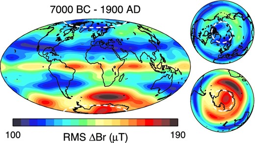
The rms radial field component (Br) residuals at the core mantle boundary (CMB) between 1000 different reference field models and models constrained by associated synthetic data sets for every 50 yr between 2000 BC and 1900 AD (see text for a more detailed description). The dashed white lines show the CMB expression (∼71° N/S) of the inner core tangent cylinder.
Not surprisingly the largest rms Br residuals are observed at high latitudes, particularly in the Southern hemisphere beneath Africa and the Pacific, related to the occurrence of high intensity flux patches. The least difference is observed at mid-latitudes around the northern hemisphere and beneath South America and the SW Pacific where the data distribution is most dense. The low misfit recorded at very high latitudes in the Northern hemisphere is probably a combination of little temporal variability in the reference model due to the rotation around the Earth's axis and the fact that the available data, in particular field intensity, sample the field quite well at the CMB, where we apply our regularization (see fig. 1 of Korte et al.2011).
Comparing the temporal variability of the initial reference field model (for 1840 AD) to the corresponding synthetic model shows that the synthetic model is able to capture both high latitude high intensity flux patches in the northern hemisphere throughout the model time period. For the most part, however, the model only resolves one diffuse high intensity flux patch in the southern hemisphere. This is partially due to the location of the southern hemisphere flux patches in gufm1 for 1840 AD being situated close to each other. If we change the polarity of the reference model (gufm1 at 1840 AD) the synthetic model will at times resolve two southern hemisphere flux patches, but usually only when these are located beneath South America and the SW Pacific where there the data distribution is denser (see animation provided in the Supporting Information, mov5). This implies that we cannot discriminate between longitudinal drift and growing/weakening flux patches in the southern hemisphere, and even the long-term average persistence of flux patches could be a product of sampling bias.
A similar type of stop-and-go behaviour of the northern hemisphere high latitude flux patches observed in the palaeofield models can be observed in the synthetic models as well, although not to the same degree. This suggests that some of the stop-and-go behaviour could be an effect of the age uncertainties of the data, particularly the correlated uncertainties of the sedimentary data. There is also a tendency of flux patches seemingly appearing, or growing in intensity, as they pass beneath areas with a denser data distribution (as with the southern hemisphere comparison), suggesting that the uneven geographical data distribution could also produce a similar effect.
Fig. 11 shows time-longitude plots of all three new models and the initial synthetic model (gufm1 at 1840 AD) based on the radial field prediction for the latitude 60°N. In order to emphasize azimuthal structure of the field we also show time-longitude plots after removing the time-averaged axisymmetric part of the field (Finlay & Jackson 2003). The westward drift of the high latitude flux patches in the northern hemisphere, noted earlier, is visible for the greater part of the last 4000 yr and looks fairly similar to the artificially induced drift of the synthetic model. Interestingly this pattern does not extend further back in time in the palaeofield models, but rather there is a hint of persistent flux patches around −60° and 60°, and possibly also around 180° E, as seen in the long-term time-averaged field (Fig. 6). The presence of the westward drift in the synthetic model throughout the model time period suggests that lack of drift in earlier part in palaeofield models is not due to problems with data distribution and/or uncertainties, but a real feature of the field.
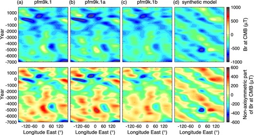
Time Longitude plots of the radial field component (Br) at the core mantle boundary (CMB) for all three new models and a synthetic model (based on the gufm1 at 1840 AD, see text for more details) centred around 60°N before (upper panel) and after removal of the time-averaged axisymmetric part of the field (lower panel).
5 CONCLUSIONS
The pfm9k spherical harmonic models represent a new family of low temporal resolution Holocene global geomagnetic field reconstructions. These are intended as alternatives to the widely used CALS10k.1b, covering the same time interval, but also as complements to higher temporal resolution field models covering the last three millennia such as ARCH3k.1, CALS3k.4, A_FM and ASDI_FM (Licht et al.2013).
All three new models show evidence for persistent high latitude high intensity flux at the CMB beneath Greenland, Western Russia, South America and the Pacific Ocean (Fig. 7). However, comparisons with models constrained from synthetic data sets show clear limitations of these predictions for high latitudes in the southern hemisphere. One of the most striking features of the time evolution of the field at the CMB, predicted by all three new models, is a dominant westward motion of northern high latitude high intensity flux patches around the edge of the tangent cylinder during the last 4000 yr. These results are in contrast to similar studies where both westward and eastward drift has been observed to be more or less equally common over the same time period (Dumberry & Finlay 2007; Wardinski & Korte 2008; Amit et al.2011). We find that a combination of the increased weight given to intensity data, which preferentially samples higher latitudes at the CMB (Johnson & McFadden 2007), and the inclusion of high latitude sedimentary declination data (Barletta et al.2008; Lisé-Pronovost et al.2009) are important for tracking the motion of these high latitude flux patches. The new models also show intermittent occurrences of reversed flux at the edge of or inside the tangent cylinder, possibly originating from the equator, but further investigations are required to determine how robust these features are.
The new models are based on essentially the same data as CALS10k.1b but introduce new ways of treating the data, particularly sedimentary data. These include redistributing the weight given to different sources and types of data during the inversion as well as addressing their chronologic uncertainties in a novel way. We find that the single most important change is the resampling of the sedimentary data, effectively reducing the influence of a few individual records that dominated the field reconstructions for some regions of the world, but also reassigning more weight to archaeomagnetic data and data based on more measurements. In future studies, more comprehensive approaches could be used to further distinguish between records based on sedimentation rates and quality estimates such as the scatter of data from different independently oriented cores (Nilsson et al.2010; Panovska et al.2012).
Appropriately treating the sedimentary declination data as relative values has a large impact on the final model outcome, particularly for regions such as the SW Pacific where the models are dominantly constrained by sedimentary data. As discussed in Section 4.2 the adjustments used here may have led to a slight transfer of power from higher degrees into the dipole component. We conclude that adjustments to the declination data are necessary but that the methodology could be improved. Similar adjustments may also be appropriate for the sedimentary inclination data, which in a few cases appear to be systematically offset by more than 10° based on comparisons with archaeomagnetic data. Like Panovska et al. (2012) we did not observe any systematic evidence of inclination shallowing and decided against adjusting the inclination data to avoid removing real persistent non-dipolar features. We note, however, that just by resampling the data most erratic offsets in either (un-adjusted) declination or inclination were successfully identified and removed as outliers by the modelling procedure.
One of the main problems associated with geomagnetic field modelling using sedimentary palaeomagnetic data are the large and often unknown age uncertainties. In the most recent modelling efforts this problem has been approached by bootstrap resampling of the data set, see Section 3.3, whereby one part consists of shifting the whole chronology of each sedimentary record randomly in time by a fixed value of ±300 yr (Korte et al.2009) or using the smaller published age uncertainties (Licht et al.2013). Here we have instead introduced an alternative, and arguably more realistic, way of adjusting the sediment data chronologies by randomly stretching and compressing the individual timescales of each record. Using this technique we have both been able to assess the likely range of age uncertainties, often up to and most likely also exceeding 500 yr, and adjust the timescale of each record based on comparisons with predictions from pfm9k.1. There are obvious limitations with the methodology applied here, mainly the implicit assumption that the pfm9k.1 is free of chronologic errors. Yet, the results demonstrate the potential information stored in sedimentary data, which can be recovered using the stratigraphic information provided with each record. Temporal smoothing and time-lag related to lock-in processes may also be important but we find that chronologic uncertainties are most likely of greater concern for geomagnetic field reconstructions based on sedimentary data.
The source files for all three models, including the pfm9k.1b individual bootstrap solutions, together with evaluation software are provided in the EarthRef.org Digital Archive (ERDA, http://www.earthref.org) by searching for the model names.
This work was funded by the Natural Environment Research Council, UK, grant numbers NE/I013873/1 and NE/H021043/1. MK acknowledges support from grant KO 2870/4–1 of Deutsche Forschungsgemeinschaft. We thank Catherine Constable and an anonymous reviewer for their constructive reviews of the original manuscript.
REFERENCES
SUPPORTING INFORMATION
Additional Supporting Information may be found in the online version of this article:
Movie 1.
Movie 2.
Movie 3.
Movie 4.
Movie 5. (Supplementary Data)
Please note: Oxford University Press is not responsible for the content or functionality of any supporting materials supplied by the authors. Any queries (other than missing material) should be directed to the corresponding author for the article.
