


Abstract
We use the method of simultaneously encoded sources to perform computationally inexpensive full-waveform inversion (FWI) on fixed-spread, marine seismic data. A workflow is proposed whereby both data- and model-based preconditioning strategies are enforced to mitigate the non-linearity of the seismic inverse problem. Artificial crosstalk, introduced by the false correlation of forward and adjoint wavefields of simultaneously simulated sources, is minimized by simulating supershots of random linear combinations of data with iteration-varying encoding. Using encoded sources with partial-source assembly, crosstalk is furthermore suppressed by randomizing the locations of encoded subsources. Synthetic case studies verify our basic workflow approach, demonstrating accurate model reconstruction in the most extreme case of a single supershot. Application to real data from the Valhall oilfield in the North Sea demonstrates reconstruction of near-surface features with one to two orders of magnitude speedup per FWI iteration. Such an efficiency gain can be incorporated into a seismic data processing workflow both for tomographic inversion and for quality control measures.
1 INTRODUCTION
Full-waveform inversion (FWI) has emerged as an effective method for delivering high-resolution tomographic images of the Earth's structure. Although the theoretical foundation for FWI has been known for several decades (e.g. Tarantola 1984), only in recent years have available computing resources caught up to the demands of fully 3-D FWI at the exploration scale (e.g. Plessix 2009; Sirgue et al. 2010; Vigh et al. 2010; Etienne et al. 2012). Such applications may still consume 104–106 CPU hours per FWI iteration, however, pushing the limits of institutional computer clusters. FWI is furthermore hindered by a general lack of robustness with respect to arbitrary starting model and inversion workflow: typically, preconditioning strategies (both in data and model domains) are required for FWI to converge to physically plausible models. By lowering the cost per FWI iteration, one could speed up the cycle of workflow testing and development. This forms the motivation for the present study.
FWI is posed as an optimization problem, the goal of which is to derive a seismic velocity model that minimizes misfit between observed and synthetic seismograms. Typically, iterative methods are deployed in which the gradient of misfit with respect to model parameters is calculated to yield a model update direction. Calculation of the gradient requires computation of at least two (forward and adjoint), and possibly more, numerical simulations of the seismic wave equation per source per FWI iteration. Marine seismic acquisition systems at the exploration scale typically have order tens to hundreds of thousands of sources, thus posing a formidable computational bottleneck. Acceleration of this component of the inversion, therefore, has potential to significantly reduce overall cost.
Recently (Capdeville et al. 2005; Vigh & Starr 2008; Krebs et al. 2009; Boonyasiriwat & Schuster 2010; Baumstein et al. 2011; Ben-Hadj-Ali et al. 2011; Routh et al. 2011), simultaneous-source methods have been investigated as a means to reduce this cost, by exploiting the linearity of the governing wave equation with respect to source terms to reduce the total number of simulations per FWI iteration. ‘Source encoding’, as is commonly referred to in the literature, reduces the cost of each FWI iteration by a factor approximately equal to the number of simultaneous shots per supershot. The resulting inverted velocity model, however, suffers from crosstalk artefacts due to the (false) correlation between forward and adjoint wavefields of shots encoded within a common supershot. These artefacts can be partially mitigated by encoding shots via incoherent summation (Krebs et al. 2009; Ben-Hadj-Ali et al. 2011), incoherent source locations (Boonyasiriwat & Schuster 2010) and preconditioning of the gradient search direction (Guitton & Diaz 2011).
It has been argued (van Leeuwen & Herrmann 2013) that the overall convergence rate of encoded-source FWI (with respect to number of wave equation simulations) is not demonstrably faster than conventional, serial-source FWI with batching strategies. In the latter approach, a subset of serial sources is drawn without replacement for each iteration. Regardless, encoded-source FWI offers potential for orders of magnitude speedup on a per-iteration basis, allowing for fast computation of the misfit functional and its gradient (albeit with less resolution). We believe therefore that encoded-source FWI could be considered as a standard tool in fixed-spread FWI workflow. Baumstein et al. (2011) reported successful application to field data, inverting surface waves for shear velocity model update. To our knowledge, however, rigorous studies of encoded-source FWI have yet to be performed.
In this paper we demonstrate the success of encoded-source FWI applied to fully 3-D models in both synthetic and real-data cases at the exploration scale using a time-domain numerical solver. The paper is organized as follows. In Section 2, we review classical FWI and the method of source encoding. In Section 3, we detail a specific workflow implementation for encoded-source FWI, where preconditioning in both data- and model-domains is applied. In Section 4, we verify our workflow against synthetic tests, demonstrating accurate model reconstruction even in the limiting case of a single encoded supershot, and consider sensitivity of the inverted model with respect to various workflow strategies. In Section 5, we apply the workflow to ocean-bottom cable data from a survey of the Valhall oilfield in the North Sea, demonstrating that one to two orders of magnitude speedup per FWI iteration may be possible via encoded simultaneous sources.
2 BACKGROUND
2.1 Acoustic-wave propagation
The acoustic approximation is typically limited to marine settings, where surface wave effects (e.g. ‘ground roll’) are minimal in comparison to land data. Soft-seabed marine environments prevent significant P–S conversions, while hydrophone receivers do not record S waves. Brossier et al. (2009) and Barnes & Charara (2009) demonstrate the feasibility of acoustic FWI in soft-seabed environments.
Although seismic waves are known to be sensitive to comparatively complex media in the Earth (e.g. elasticity, anisotropy and viscoelasticity), the acoustic approximation remains the standard model parametrization for exploration-scale FWI due to cheap numerical cost and high sensitivity to acoustic waves. Furthermore, the results of Sirgue et al. (2010), in which FWI was applied to OBC data from the Valhall field, demonstrate that remarkably high-resolution tomographic images can be recovered even in the approximation of an acoustic isotropic medium.
2.2 Full-waveform inversion
The seismic inverse problem seeks to compute a seismic velocity model by minimizing differences between synthetic and recorded-data waveforms. Classically, ray-theoretical methods have been used to invert for the Earth's structure, relying upon simplified assumptions of the starting model medium and utilizing a small amount of information per waveform (such as traveltimes of distinct phases). An alternative approach is FWI, which can potentially utilize information from the entire waveform. Application of FWI requires no assumptions with respect to starting model, although a sufficiently accurate starting model is needed to avoid cycle-skipping artefacts (see e.g. Virieux & Operto 2009; Prieux et al. 2013c).
2.3 Simultaneous-source methods
Although exploration-scale FWI applications have a smaller physical model to consider than their global-scale counterparts, the total number of events to simulate in the former case (e.g. airgun sources) typically dwarfs the latter (e.g. earthquakes). Each iteration of FWI minimally requires two numerical simulations of the wave equation (forward and adjoint) per source event, with additional simulations over a subset of sources possibly necessary for calculation of the step length and/or Hessian matrix. Conventional FWI therefore may require tens to hundreds of thousands of numerically expensive wave equation simulations per iteration. Although the cost per simulation can vary significantly whether one adapts a time- or frequency-domain discretization of the wave equation, the underlying bottleneck posed by many sources remains.
The main drawback of simultaneous source methods is crosstalk artefacts, introduced by the false correlation of encoded forward and adjoint wavefields in gradient calculations. Choosing random (i.e. incoherent), iteration-varying codes, however, reduces crosstalk noise by averaging it away over successive FWI iterations. This was the key discovery from Krebs et al. (2009), where a time-domain implementation with random codes |$c_n^{(i)} = \pm 1$| was demonstrated to deliver high-accuracy models with a single encoded supershot. Ben-Hadj-Ali et al. (2011) derived a similar approach for frequency-domain modelling, with complex-value codes chosen from the unit circle. Their studies demonstrated that encoded-source FWI is dependent upon the number of encoded supershots, number of inversion iterations and number of inverted frequencies chosen; this suggests that a fair degree of fine-tuning may be required for optimal efficiency gain. Boonyasiriwat & Schuster (2010) advocated a further degree of randomness to suppress crosstalk noise, choosing random shot locations for each supershot (e.g. |$c_n^{(i)} \in \{ - 1,0,1\}$|).
A clear restriction of simultaneous source simulation is the requirement for shots encoded within a common supershot to share the same receivers; this is violated in acquisitions with variable geometries (e.g. marine streamers). Routh et al. (2011) proposed an approach to reduce this restriction by using a cross-correlation objective functional. In this study, we restrict ourselves to fixed-geometry, ocean-bottom cable data. We utilize the time-domain implementation of encoded simultaneous sources proposed by Krebs et al. (2009) and Boonyasiriwat & Schuster (2010).
Despite demonstrated successes in encoded-source FWI, an underlying mathematical argument persists against the technique: namely, that the (iterative) non-linear optimization problem will converge slowly relative to conventional methods with non-encoded sources. This argument was advocated in van Leeuwen & Herrmann (2013), who explored the strategy of using increasingly larger subsets of the (non-encoded) sources for each FWI iteration. In our experience, the rate of misfit decrease (measured as a function of iteration number) for early-stage FWI is roughly equivalent for encoded sources and non-encoded sources; this result is reported as well in Krebs et al. (2009; their fig. 8). While at later iterations, the convergence rate of encoded-source methods may be slow relative to conventional FWI, we believe that encoded-source FWI could be used effectively to accelerate the early stages of an inversion.
3 FWI WORKFLOW
3.1 SEM discretization
The core component of a FWI workflow is the repeated numerical solution of forward and adjoint wavefields. For this task we employ the SPECFEM3D Version 2.0 ‘Sesame’ code (Peter et al. 2011), an open-source community code that models seismic wave propagation utilizing a spectral element discretization in space and an explicit Newmark scheme in time. The spectral element method (e.g. Komatitsch & Vilotte 1998; Chaljub et al. 2007; Tromp et al. 2008) is a well-known numerical scheme in the field of seismic wave propagation, combining the geometrical flexibility (h-adaptivity) of the classic finite element method with a high-order solution basis that is well-suited for wave propagation. Source terms are implemented as point forces on the Gauss–Lobatto–Legendre (GLL) gridpoints, and interpolated using Lagrange interpolants when a source coordinate does not coincide with a gridpoint. Waveforms are similarly recorded at receiver locations through Lagrange interpolation. At the free surface of the domain, a zero-pressure Dirichlet boundary condition is implemented, while at all other boundaries Clayton–Engquist absorbing conditions are applied. Non-physical (numerical) boundary reflections persist, however, acting as a source of coherent noise.
3.2 Workflow implementation
For efficient implementation of the iterative inversion process, we design a workflow (Table 1) that is intended to operate with minimal user interaction. We adopt a modular design philosophy, whereby heterogeneous workflow tasks (e.g. source encoding, kernel processing and misfit computation) are implemented and integrated with one another through Python scripts. The same scripts are used to wrap around calls to the relatively more expensive wave equation solver, which is coded in Fortran. The SPECFEM3D solver computes both forward and adjoint wavefields; in the latter case, the forward simulation is recomputed simultaneously at a reversed time from the adjoint simulation, so that sensitivity kernels may be constructed on-the-fly. The adjoint simulation is thus two to three times more expensive as the forward simulation, but we are saved the cost of having to store the forward field in memory when computing the gradient.
FWI workflow. Steps with * are computed in SPECFEM3D while all other steps are implemented in Python.
| Pre-processing: |
| 1. Encode hydrophone data via method of Krebs et al. (2009) for a sufficient number of FWI iterations |
| 2. Filter, then taper, encoded data |
| For each depth threshold: |
| For each frequency band: |
| Iterate until desired stopping criteria: |
| a) For each event: |
| 1. Compute forward wavefields* |
| 2. Compute adjoint source |
| 3. Compute adjoint wavefields (and simultaneously, sensitivity kernels)* |
| b) Sum sensitivity kernels |
| c) Precondition summed gradient search direction |
| d) (Optionally) compute step length and update model |
With typical data quantities involving hundreds of millions of recorded traces, industrial FWI applications demand efficient data processing implementations. In our workflow we integrate routines from the Obspy library (obspy.org; Beyreuther et al. 2010), a Python-based open-source toolbox for computational seismology. The Obspy library effectively standardizes our industry data set and numerically derived synthetics into a common format where all processing is performed, and subsequently fed back into the workflow. Complimenting this toolbox is the additional, stand-alone Python module pprocess (pypi.python.org/pypi/pprocess), which we utilize for trivial parallelization of signal processing operations.
Our workflow is specially designed for implementation on a Peta-scale supercomputer. Specific consideration of system architecture was necessary for efficient implementation (e.g. I/O speeds on available file systems and allocation of memory and compute tasks per node). The modular approach offered by the Python language allows for a robust workflow construction, easing the transition from institutional cluster to supercomputer.
3.3 Multiscale inversion strategies
As is common with non-linear inverse problems, FWI suffers from the presence of local minima in the objective functional, particularly when the least-squares (L2) norm (eqs 2 and 6) is adopted. The use of a gradient-based search algorithm to solve the optimization problem (eqs 2–4) is especially prone to convergence towards local minima, depending on the accuracy of the starting model. One may naturally consider preconditioning strategies in both the data- and model-space domains to mitigate the non-linearity of FWI.
It is well known (e.g. Bunks et al. 1995; Pratt 1999; Virieux & Operto 2009) that a hierarchical inversion strategy, whereby low frequencies are inverted before higher ones, can partially mitigate the tendency to converge towards local minima. This is due to the comparatively less oscillatory nature of the objective functional with respect to larger spatial wavelengths (Alkhalifah & Choi 2012). We adopt the classic time-domain multiscale strategy of Bunks et al. (1995), applying a low-pass filter to the recorded data and input source–time function. The cut-off frequency of this filter can then be incrementally varied within the FWI workflow (Table 1). In Figs 1(c) and (d) we compare the sensitivity kernels resulting from cut-off frequencies of 1.0 Hz and 6.0 Hz with an encoded-source simulation. The lower frequency cut-off results in larger spatial wavelengths in the gradient, as expected.
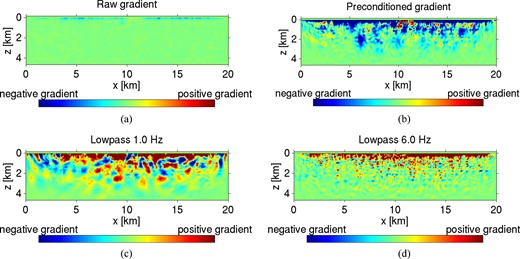
Demonstration of model-domain (a and b) and data-domain (c and d) preconditioning strategies for acoustic sensitivity kernels. (a) Raw gradient for a simulation, leaving high concentration in sensitivity near the ocean-floor receivers (150 m depth). (b) Preconditioned gradient, where an overall threshold has been applied to extend sensitivity to 1500 m depth. (c) Preconditioned gradient for an encoded source, low-pass filtering data with 1.0 Hz cut-off frequency. (d) Preconditioned gradient for an encoded source, low-pass filtering data with 6.0 Hz cut-off frequency. Colour scales for all panels are set according to the maximum absolute values for each case.
The strategy outlined by eqs (7)–(9) effectively levels all extreme values of the gradient, K(x, y, z), for regions above the depth threshold (0 < z ≤ zthreshold) to the value of the gradient threshold, K+ or K−, depending on the sign of sign of K. In Figs 1(a) and (b) we compare sensitivity kernels of an encoded-source, synthetic OBC experiment in the cases of no preconditioning and with a depth threshold of 1.5 km applied. In the former case the sensitivity is strongly restricted to the nearest 100 m below the seafloor, whereas in the latter case the preconditioned gradient contains strong sensitivity down to the depth threshold.
4 SYNTHETIC APPLICATION
To verify our workflow approach we consider synthetic application of encoded-source FWI. Synthetic testing in a controlled environment eliminates many sources of error that exist in realistic FWI applications, such as noise present in the data, unknown or poorly constrained model parameters, and unknown source wavelet. The resulting problem, albeit simplified, allows for testing of viable workflow strategies to use on real data. In our case, we consider high levels of source encoding, demonstrating that even in the maximal case of a full-source assembly (i.e. all sources simultaneously simulated), accurate model reconstruction is possible. This confirms earlier synthetic studies by Krebs et al. (2009) and Ben-Hadj-Ali et al. (2011). We furthermore demonstrate robustness of the workflow with respect to noise and starting model accuracy, before finally examining performance of partial-source assembly.
4.1 SEG/EAGE overthrust model
We perform encoded-source FWI on the synthetic 3-D SEG/EAGE overthrust model (Aminzadeh et al. 1997). An acoustic model with known, constant density is assumed for both true and initial models. 4.5 s of ‘data’ are generated by numerically simulating the wave equation on the true model. The computational grid is discretized by hexahedral spectral elements with characteristic edge length 150 m, and local polynomial degree 4 (125 local gridpoints per element). This resolution is sufficient for a minimal 2 elements per wavelength in the subsurface of the model at the highest inversion frequency (6 Hz). We use only a single element for the water layer, as a finer discretization in this region would substantially increase the numerical cost, and resolution tests demonstrated negligible change in the simulated waveforms between our chosen mesh and a refined one.
The P-wave velocity model, initially defined on a grid of 801 × 801 × 187 values and characteristic spacing 25 m, is integrated into the spectral element mesh via trilinear interpolation onto the GLL computational gridpoints. We consider this interpolated model to be the ‘true’ model. No further interpolation is required after this initial step, as the same grid is used for both model and computation (i.e. the GLL gridpoints). To mimic an ocean-bottom cable experiment, we append a 150 m water layer to the top of the model, with fixed, known velocity of 1480 m s−1. Invoking source–receiver reciprocity, we place within this water layer a square 200 × 200 array of receivers near the water surface and a 24 × 24 array of acoustic sources near the seafloor. The receivers and sources are placed equidistantly across the inner 361 km2 and 324 km2 of the model, respectively (Fig. 2). An initial model (Figs 3a–d) is derived by smoothing the true model via convolution with a Gaussian wavelet of characteristic width 300 m in the y–z plane.
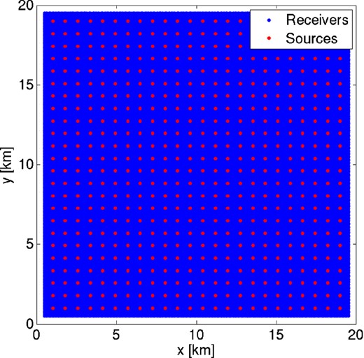
Schematic of synthetic overthrust model acquisition. 40 000 receivers (blue region) are spaced equidistantly across the inner 361 km2. 576 receivers (red dots) are spaced equidistantly across the inner 324 km2. With encoded sources we consider FWI approaches simulating all 576 sources simultaneously (Figs 3–6) and with nine supershots containing 64 simultaneous sources (Fig. 7).
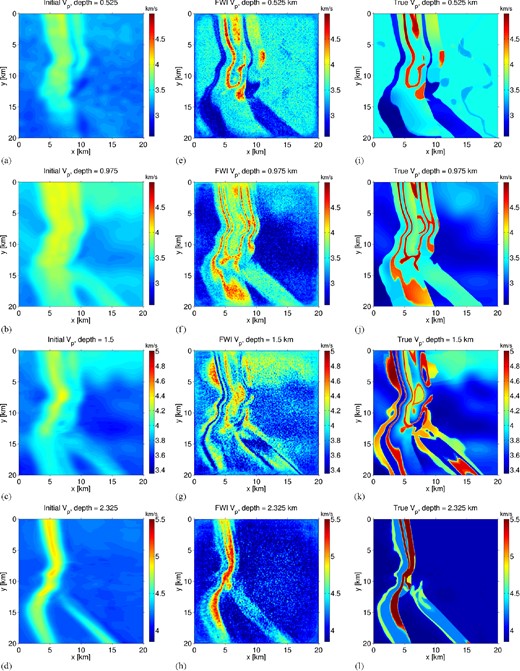
Reconstruction of synthetic acoustic overthrust model using full-source assembly. Each iteration simulates one supershot containing 576 encoded sources; (a–d) starting model, formed by smoothing the true model; (e–h) FWI-derived model; (i–l) true model. Final model (L1-norm) error is approximately 65 per cent of starting model error.
4.2 Results encoding 576 shots into one supershot
We implement encoded-source FWI with full-source assembly, achieving maximal speedup per inversion iteration by encoding all sources into a single supershot. 130 FWI iterations are performed with a gradient descent method and fixed step length of 2.5 per cent. Although this represents a simplistic approach to solving the non-linear optimization problem, the goal of this study is to focus on the efficiency of encoded-source FWI, and so we prefer to choose simpler strategies wherever possible in the inversion workflow. With respect to the workflow detailed in Table 1, we apply a low-pass filter with sequentially larger cut-off frequencies of 1.0, 1.5, 2.5, 4.0 and 6.0 Hz, performing 10 iterations per frequency. Initially we choose a gradient threshold depth at 1.5 km. At iterations 50 and 100, the threshold depth is increased to 2.25 and 3 km depth, respectively. The inversion is manually terminated when the rate of model and data misfit become negligible, so we do not invert the two highest frequencies at 3 km depth.
Results of initial, FWI-derived and true acoustic velocity models are given for variable depths in Fig. 3. Low-amplitude, short-wavelength noise in the velocity models is consistent with previous numerical study of source encoding methods (Krebs et al. 2009; Ben-Hadj-Ali et al. 2011), and is attributed to crosstalk noise among the encoded sources. Despite these features, the recovered model is very highly accurate in shallower (<1 km) depths, effectively reconstructing high-contrast interfaces as well as volumes. At greater depths, interfaces are still accurately imaged, but volume information suffers. We acknowledge that our results are favourably biased, however, by including low frequencies. In Fig. 4 we consider a model slice in the x–z plane. Although the crosstalk artefacts are again present in the reconstructed model, reflecting interfaces are well-reconstructed to 3 km depth. A well log (Fig. 4d) demonstrates overall accuracy in the model reconstruction, but with significant overshoots due to the crosstalk, particularly in the upper 1.5 km.
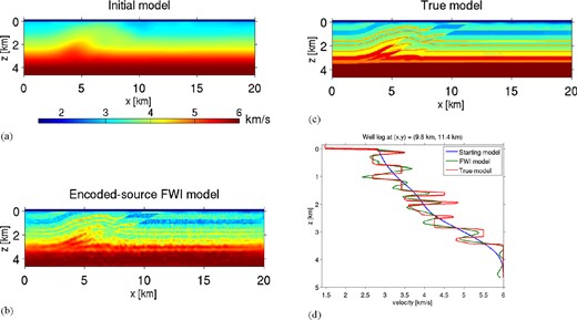
Cross-sections of the (a) initial, (b) inverted and (c) true models corresponding to the synthetic encoded source FWI of Fig. 3 at y = 11.4 km. (d) Well log for these models.
In Fig. 5 we show waveforms computed from the models in Figs 3 and 4, for a single source (Figs 5a, c and e) and for a supershot of 576 encoded sources (Figs 5b, d and f). For each source type we show data simulated from the true model, and initial and final data residuals for 200 receivers along a line. The single source yields a conventional shot record, whereas the supershot yields a complicated wavefield with no visual clarity after the direct arrivals. Misfit decrease is nonetheless clear in each case, with total misfit over the entire data space decreasing approximately 85 per cent throughout the course of the inversion. Characteristic traces (Fig. 5g) for both source types reveal a reduction in phase and amplitude misfit throughout the entire time window. We note with caution that the initial model for tests displayed in Figs 3–5 is quite accurate, yielding a higher accuracy final model than would be reasonably expected for a similar setup on real data and poor starting model.
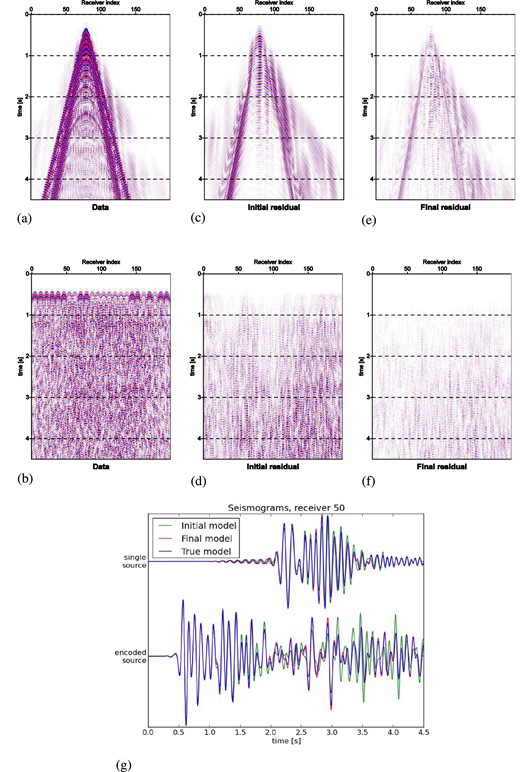
Seismogram misfit decrease demonstrated for single-source (a, c and e) and encoded-source (b, d and f) waveforms from synthetic inversions of Figs 3 and 4. (a and b) Data simulated from true model; (c and d) waveform residuals from initial model; (e and f) waveform residuals from final model, derived by encoded-source FWI; (g) single traces corresponding to receiver index 50 simulated on initial, FWI-derived and true models. Waveforms are computed along a constant line of receivers with spacing 95 m. The same colour scale is used across panels (a, c and e) and (b, d and f).
Due to the high level of encoding we have applied, the blended waveforms in Fig. 5 lack any easily identifiable signal beyond the direct arrivals. Consequentially, standard tools in time-domain FWI, such as time windowing to extract and invert for specific phases, are not at our disposal (though such tools might partially be applicable when using a less ambitious, partial-assembly encoding strategy). Regardless, our basic goal to speed up the FWI workflow as much as possible, while still yielding reasonably high accuracy for the reconstructed models, succeeds. Despite the complexity introduced through the simulation of blended waveforms, our results in Figs 3 and 4 indicate that tomographic inversion remains possible on these waveforms, at least when sufficiently low frequencies are available.
4.3 Encoded-source FWI sensitivities: noise, starting model and source assembly strategy
The inverted velocity models in Figs 3 and 4 contain (perhaps) surprisingly high accuracy, given that with full-source assembly we are applying the most ambitious form of source encoding. However, in this controlled synthetic experiment, we have bypassed some of the more realistic challenges that would be expected in real data: noise in the data, which amplifies the effect of crosstalk noise from encoded sources (Ben-Hadj-Ali et al. 2011), and a low-accuracy starting model, which could require more iterations towards convergence and/or the tendency to converge towards a less accurate final model. In Fig. 6 we demonstrate these effects by modifying the setup from Figs 3–5, considering the first 50 iterations (Fig. 6a). Fig. 6(b) repeats the baseline inversion but with a less accurate starting model, computed by smoothing the true model by a 3-D Gaussian with characteristic length 500 m. In this example, high-velocity artefacts are introduced in the near surface, as well as a generally poorer overall model reconstruction. Fig. 6(c) repeats the baseline experiment, but adds white noise to the data with characteristic signal-to-noise ratio of 5.0.
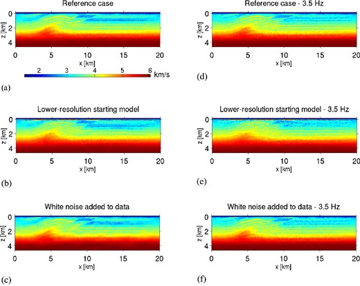
(a) Model after 50 iterations, applying same workflow as in Figs 3–5. (b) Same as (a) but with a less accurate starting model; note that high-velocity artefacts are present in the near-surface. (c) Same as (a) but with white noise added to data. (d) 50 iterations are performed with lowest inverted frequency 3.5 Hz. (e) Same as (d) but with a less accurate starting model. (f) Same as (d) but with white noise added to data.
Results in Figs 3 and 4 utilized information at low frequencies (<3.5 Hz), which typically, for field data, contain unacceptable signal-to-noise ratio for FWI. A more realistic case is considered by removing low-frequency content from the data. In Fig. 6(d) we perform 50 encoded-source FWI iterations, applying bandpass filter to invert for 3.5–4.5 Hz data, and then 3.5–6.0 Hz (25 iterations each). This result can be compared with the frequency-domain study from Ben-Hadj-Ali et al. (2011), which used starting frequency 3.5 Hz. As expected, omitting low frequencies leads to less accurate reconstruction of bulk structure, although interfaces are still aligned correctly. Figs 6(e–f) replicates the workflow of Fig. 6(d), but with poorer starting model and white noise added to data, respectively. Results are consistent with Figs 6(b and c), with a notable exception: noisy-data inversion (Figs 6c and f) appears to more severely impact the lower frequency inversion than the higher frequency one. This result was also discussed by Ben-Hadj-Ali et al. (2011), who concluded that crosstalk noise is more sensitive at lower frequencies. Model errors for all studies in Fig. 6 are shown in Table 2.
| Initial model | 1.0–6.0 Hz FWI (Figs 6a–c) | 3.5–6.0 Hz FWI (Figs 6d–f) | |
|---|---|---|---|
| Reference case | 100.0 | 81.1 | 87.9 |
| Lower resolution starting model | 109.6 | 102.2 | 107.0 |
| White noise added to data | 100.0 | 84.9 | 88.0 |
| Initial model | 1.0–6.0 Hz FWI (Figs 6a–c) | 3.5–6.0 Hz FWI (Figs 6d–f) | |
|---|---|---|---|
| Reference case | 100.0 | 81.1 | 87.9 |
| Lower resolution starting model | 109.6 | 102.2 | 107.0 |
| White noise added to data | 100.0 | 84.9 | 88.0 |
Noise present in (non-encoded) data is known to amplify the effects of crosstalk noise (Krebs et al. 2009; Ben-Hadj-Ali et al. 2011), which is proportional to the number of encoded shots per supershot. In between the extremes of full-source assembly and traditional serial sources exists a middle ground, partial-source assembly, whereby a number of supershots with fewer encoded sources are simulated. Ben-Hadj-Ali et al. (2011) studied this case in detail, demonstrating that fine-tuning may be required to reach the optimal level of speedup versus accuracy in the inverted model. In Fig. 7 we show results using partial-source assembly with nine supershots, each of which consists of 64 encoded subsources. When using a partial source assembly strategy, one must partition the total number of sources into subsets of encoded subsources. We consider three types of partitioning strategies: line-indexed (Figs 7a and d), random (Figs 7b and e) and coarsely spaced (Figs 7c and f). Line-indexed sources are chosen simply according to their index location on file, random source locations are chosen by randomly drawing 64 of the 576 indices (similar to the method of Boonyasiriwat & Schuster 2010) and coarsely spaced locations are chosen by maximizing the average spacing between sources. Random source locations are regenerated each iteration, whereas the other two are held fixed throughout the inversion (although still with random codes).
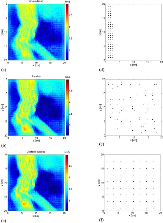
Study of source partitioning strategies for encoded-source FWI using partial-source assembly. 576 serial sources are partitioned into nine supershots of 64 encoded subsources. Model cross-sections for three partitioning strategies are shown in (a)–(c); subsource locations of the first supershot are shown in (d)–(f); (a and d) Line-indexed sources, where subsource locations are chosen according to their index on file; (b and e) random sources, where each subsource is randomly drawn in each iteration; (c and f) coarsely spaced sources, where subsource locations are chosen to maximize their average distance. L1-norm model errors for (a), (b) and (c) have reduced from initial model approximately 8, 12 and 12 per cent, respectively.
Adjacent to each model profile in Fig. 7, the location of the 64 encoded subsources for the first supershot is shown. We show the reconstructed models after 15 FWI iterations, so as to fairly compare the progress of each inversion relative to the amount of computational work done. The poorest result is delivered with line-indexed sources, where subsources are chosen simply according to their index location on file, leading to poor azimuthal illumination of the seismic ray paths. In this case, the model error has decreased approximately 8 per cent from the starting model. The models constructed from randomly chosen or coarsely spaced subsources, however, are quite similar; each has reduced the model error approximately 12 per cent from the starting value (coarsely spaced was slightly better, but due to the randomness involved we cannot make a general inference). We infer from these results that interference from closely spaced encoded sources is a primary driver of crosstalk error when using partial-source assembly.
Comparable model resolution to the results in Fig. 7 but with application of full-source assembly (not shown) was found after 67 FWI iterations, a computational cost of less than 50 per cent of that required for partial-source assembly when considering the total cost per iteration involved. It is not surprising that with noise-free synthetic FWI, the greatest efficiency gain occurs with full-source encoding (similar results were reported by Ben-Hadj-Ali et al. 2011). This result furthermore advocates that comparable resolution may be generally achieved with less computational effort when using encoded sources versus conventional, serial sources. We demonstrate this result next on real data from the Valhall field.
5 APPLICATION TO OCEAN-BOTTOM CABLE DATA FROM THE VALHALL OILFIELD
Having verified our encoded-source FWI workflow approach through synthetic tests and gained insight into the sensitivities of varying encoding strategies, we next consider application to ocean-bottom cable data from the Valhall oilfield. An ocean-bottom cable array at Valhall was installed in 2003 (Kommedal et al. 2004), comprising 45 km2 of coverage of four-component sensors embedded in the (70 m deep) seafloor. 2302 receivers are spaced approximately 50 m apart within each of the 12 cable lines, and cables are approximately 400 m apart. Hydrophone data from a survey containing 49 954 shots at maximal offset of 13 km, and an initial acoustic velocity model (derived from VTI reflection traveltime tomography and converted into NMO velocity), have been provided by BP. Density is held fixed throughout the inversion, and derived from the initial P-wave velocity model via Gardner's relation (Gardner et al. 1974), |$\rho = 310\,V_p^{0.25}$|. We model acoustic-wave propagation with a hexahedral mesh consisting of elements of approximate dimension 130 × 130 × 70 m3 in the water layer and 130 × 130 × 200 m3 in the subsurface. Source–receiver reciprocity is invoked during the numerical modelling; the ‘sources’ from this perspective are the 2302 hydrophones. A schematic of the acquisition geometry is given in Fig. 8.
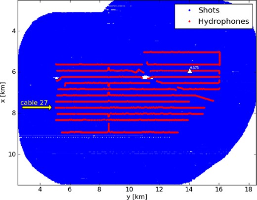
Schematic of Valhall field array acquisition, with 2302 ocean-bottom cable (OBC) hydrophones and 49 954 shots. Triangle marker denotes hydrophone 375. The 200 hydrophones from cable 27 are used to invert the source wavelet (Fig. 9). Characteristic hydrophones spacing is 50 m inline and 400 m crossline. Characteristic shot spacing is 50 m.
Acoustic isotropic FWI of the Valhall field was performed by Sirgue et al. (2010), demonstrating a network of high-velocity channels at 175 m depth and extension of a gas-filled fracture extending from a gas cloud at 1050 m depth. These features were confirmed in later studies by de Ridder & Dellinger (2011), who used ambient noise tomography to image the near-surface, and Etienne et al. (2012), who performed 3-D FWI by modelling in the time domain and inverting in the frequency domain.
Significant anisotropy is known to exist in the Valhall field (Barkved et al.2003; Olofsson et al. 2003), the effects of which will bias reflector positions (and more generally, the entire velocity model) reconstructed by isotropic FWI (Prieux et al. 2011; Gholami et al. 2012). Regardless, acoustic isotropic modelling remains a valuable tool in seismic imaging, both for purposes in generating background velocity models for depth migration (Sirgue et al. 2010) as well as for geostructural interpretation (Prieux et al. 2011). A multiparameter hierarchical 2-D FWI was followed by Prieux et al. (2013a,b) on the Valhall field to recover in cascades the compressive and shear wave speeds, the density and the attenuation. Our workflow can be of special interest to accelerate each step, in particular acoustic velocity inversion, constituting a hierarchical multiparameter inversion.
5.1 Source–time function inversion
The source wavelet is an unknown parameter in the inversion and must be reconstructed as a preliminary stage to our time-domain FWI workflow. Furthermore, the ‘raw’ data we start with have actually been pre-processed, although the details of this pre-processing are not available to us. Pre-processing effects are most notable by the non-causal nature of the nearest offset traces (Fig. 9f), and a (coarse) time sampling of 32 ms in each shot record. All data pre-processing is absorbed into the inverted source wavelet.
![(a–c) Inverted source wavelet across 200 hydrophones of cable 27 (see Fig. 8) using the workflow in Table 2 applied to 3, 10 and 100 nearest source–receiver offsets. (d) Averaged, normalized source wavelet across all hydrophones in (a)–(c). (e) Spectrum for wavelets in (d). (f) Raw data from hydrophone number 375 (see Fig. 8) for a horizontal line of shots; unknown pre-processing operations have been applied. (g) Reprocessed data from (f), where a bandpass Butterworth filter with cut-off frequencies [2.0, 4.0] Hz and a cosine taper have been applied. (h) Synthetics computed from the initial model and source–time function from (d) derived by averaging wavelets inverted by the nearest (three traces) offsets; note that we observe numerical artefacts relating to source implementation and boundary reflections. The same colour scale is used for (f)–(h).](https://oup.silverchair-cdn.com/oup/backfile/Content_public/Journal/gji/195/3/10.1093/gji/ggt362/2/m_ggt362fig9.jpeg?Expires=1716348300&Signature=g3ioN0Ogfnf39nHylZBZwH9hpkVOU~SnTpRYqRiGURl2EpU8jDyBwgy60pc5v0uEQuZ0ID0YBFUewYx-58iyqR7n0wAhg7rxlPo9gnj4otrexeLgPE7VHsw77IgI7iTq-0qaQMHz62~RHQl-Tms~ckcfK4GjSzeSQ6TpKpirzljH3LmrTeSbP928-n5dUxtThogrot0atM8B79sBHG-s40OMY1-VqABEqjQdzpv9Dd01-N7UNbdXUSzoOUoVUxJFYjaXTPvU8dL7gvZ5coEZYVGw~uC2G8YCVV1xR3qOpiIA5vu3ahvRcvcMNfrb6oV67zFBnaC6dNHWW3bGBOGM1Q__&Key-Pair-Id=APKAIE5G5CRDK6RD3PGA)
(a–c) Inverted source wavelet across 200 hydrophones of cable 27 (see Fig. 8) using the workflow in Table 2 applied to 3, 10 and 100 nearest source–receiver offsets. (d) Averaged, normalized source wavelet across all hydrophones in (a)–(c). (e) Spectrum for wavelets in (d). (f) Raw data from hydrophone number 375 (see Fig. 8) for a horizontal line of shots; unknown pre-processing operations have been applied. (g) Reprocessed data from (f), where a bandpass Butterworth filter with cut-off frequencies [2.0, 4.0] Hz and a cosine taper have been applied. (h) Synthetics computed from the initial model and source–time function from (d) derived by averaging wavelets inverted by the nearest (three traces) offsets; note that we observe numerical artefacts relating to source implementation and boundary reflections. The same colour scale is used for (f)–(h).
Workflow for source–time function inversion.
| I. For each hydrophone: |
| 1. Compute Green's functions g for nearest traces |
| 2. Bandpass filter d with cut-off frequencies [2.0, 4.0] Hz |
| 3. Compute Fourier transform of g and d. |
| 4. Deconvolve each frequency, per eq. (11) |
| 5. Compute inverse Fourier transform of resulting wavelet |
| 6. Apply cosine taper |
| II. Average all inverted source–time functions |
In Fig. 9 we invert for the source wavelet over receiver gathers, considering 200 hydrophones of cable 27 (see Fig. 8) using the nearest 3, 10 and 100 shots to each hydrophone (Fig. 9d). The wavelet is derived then by stacking the 200 individual wavelets in each case. Our approach notably uses far fewer traces than the study of Prieux et al. (2011), who considered offset ranges of 2–13 km when inverting the source wavelet. When using the fewest number of traces, artefacts are observed in the wavelets constructed from hydrophones near the cable edges (in particular for hydrophones 0–10). As these artefacts disappear by increasing the number of traces included in the wavelet reconstruction, we interpret their presence as due to local, coherent noise (either real or numerical) present in the inverted frequency bands. Conversely, including more traces increases the likelihood of model structure being mapped into source wavelet, as shallow-water refractions sampling the near-subsurface are included in the data set. Our numerical experiments indicated this latter issue to be a greater overall concern: data misfit was lowest when using the wavelet computed from the smallest number of offsets, and reconstructed models had greater overall clarity and resolution. Therefore we select the wavelet derived by averaging Fig. 9(a) as our source–time function.
We simulate data with the selected source wavelet on hydrophone 375, comparing against data that is reprocessed with the same workflow as the source wavelet (Figs 9g and h). At nearest offsets we observe a close match with synthetics, whereas for farther offsets we observe cycle skipping in first arrivals (see also Figs 12b and d). This is due to a general failure of the NMO-derived acoustic isotropic starting model to accurately honour the kinematics of the medium; in particular, for large-offset diving waves. For a discussion and appraisal of varying starting model choices we refer to Prieux et al. (2011). We note also numerical artefacts in our modelling in Fig. 9(h): boundary reflections are observed for 0–5 km offsets and 4–5 s time window, and ‘triangle’-shaped features at near-zero offsets are likely due to source artefacts in the thin water layer.
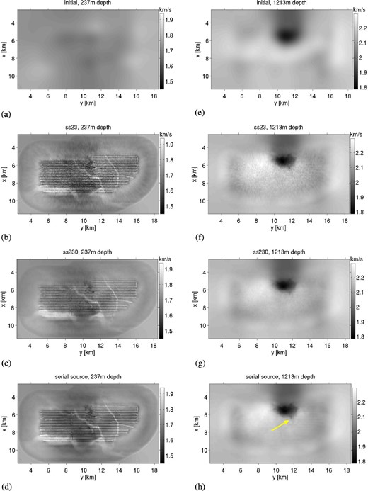
Encoded-source FWI of the Valhall oilfield, with velocity model cross-sections at depths (a–d) 234 m, where a network of high-velocity channels are observed, and (e–h) 1200 m, where low-velocity extension of a gas cloud is observed (yellow arrow). Both of these model features are reported in the previous works of Sirgue et al. (2010) and Etienne et al. (2012). (a and e) Initial model; (b and f) 23 supershots per iteration (ss23), each containing 100 encoded sources; (c and g) 230 supershots per iteration (ss230), each containing 10 encoded sources; (d and h) 2302 sources per iteration with no encoding.
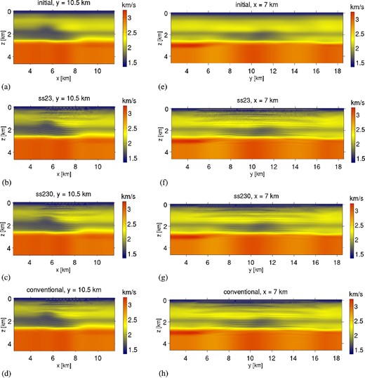
Encoded-source FWI of the Valhall oilfield: x–z cross-sections (a–d) and y–z cross-sections (e–h). (a and e) Initial model; (b and f) 23 supershots per iteration (ss23), each containing 100 encoded sources; (c and g) 230 supershots per iteration (ss230), each containing 10 encoded sources; (d and h) 2302 sources per iteration with no encoding. Similar layered interfaces are observed with each encoding scheme, but ss23 contains notably larger crosstalk noise, as well as greater acquisition footprint.
![Waveform residuals for the Valhall inversion computed from initial model (a) and final model (c), the latter of which was derived from partial-source assembly strategy ss23. Inline traces for hydrophone 375 (see Fig. 8) are shown. The same colour scale is used. (b) Near-offset traces shown convergence in early (<1.5 s) arrivals but acoustic FWI fails to fit the (elastic) Scholte wave (1.5–2.25 s). (d) Cycle-skipped at farther offsets. Traces in (b–d) correspond to the derived models in Figs 10 and 11. All traces are bandpass filtered over [2.0, 4.0] Hz.](https://oup.silverchair-cdn.com/oup/backfile/Content_public/Journal/gji/195/3/10.1093/gji/ggt362/2/m_ggt362fig12.jpeg?Expires=1716348300&Signature=hhBIM4X9N8Ga1T6l~gsrXCeSFP97X-1cgJ0XRP96Lo2H~FOo3cwG3qJcEcLKHUAFSpD9w0av9VCBApS3IqQXeNeaSdA1togHaO2EWW7hn1DjepazwmeVS~PONOB81QTkE8l9eQlYs2ZOexyRm2cc7UQO7gWwtaMV-dWNt3lLuubQ0SHqT6BoxV2YGyo5uT-ZL5bYp5r3lL9iCRKwPVJJmQdYgZ6thDIu81YSRjJhVq-hPZPWeQOuiO2m3tzKbGc0hfG1DiWBFp8LHMm4OzKAFkdnib4hfg3jBW4kVdPITnCZTF2-~dhrKS15btbbAuuGhPwR1P0sFFQi1vbyIbnxvQ__&Key-Pair-Id=APKAIE5G5CRDK6RD3PGA)
Waveform residuals for the Valhall inversion computed from initial model (a) and final model (c), the latter of which was derived from partial-source assembly strategy ss23. Inline traces for hydrophone 375 (see Fig. 8) are shown. The same colour scale is used. (b) Near-offset traces shown convergence in early (<1.5 s) arrivals but acoustic FWI fails to fit the (elastic) Scholte wave (1.5–2.25 s). (d) Cycle-skipped at farther offsets. Traces in (b–d) correspond to the derived models in Figs 10 and 11. All traces are bandpass filtered over [2.0, 4.0] Hz.
5.2 Encoded-source FWI of the Valhall field
Having constructed a suitable source wavelet, we now apply our FWI workflow to the Valhall data set. We compare our results to the previous studies of Sirgue et al. (2010) and Etienne et al. (2012), where a network of high-velocity channels in the shallow subsurface are observed (their figs 3 and 9, respectively), and a gas-filled fracture extending from a gas cloud at depth is observed (their figs 3 and 4, respectively). We consider partial-source assembly with encoded sources of 23 and 230 supershots (henceforth denoted ‘ss23’ and ‘ss230’), equating to per-iteration cost reduction of two and one orders of magnitude, respectively. We examine reconstructed models from iterations 6 and 16 for the partial-source assembling strategies ss230 and ss23, respectively; misfit decrease was negligible for later iterations (Fig. 14). Therefore the overall cost of ss23 was approximately 3.75 times cheaper than the cost of ss230, and approximately 6.25 times cheaper in total than a single iteration of serial-source FWI. We invert for the first 4 s of data, as later arriving waveforms are dominated by Scholte waves at near offset and cycle-skipping artefacts at long offsets; both of which cannot be accurately accounted for in our acoustic isotropic model. A depth threshold of 1050 m is used for gradient preconditioning, chosen to enhance sensitivity of the model update near the gas cloud. The model is updated according to the (preconditioned) steepest-descent direction with constant step length 2.5 per cent.
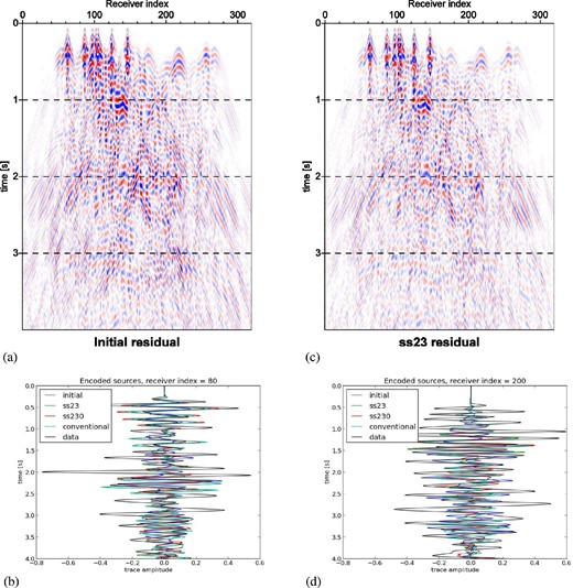
Waveform residuals for the Valhall inversion computed from initial model (a) and final model (c), the latter of which was derived from partial-source assembly strategy ss23. A supershot of 100 encoded sources is simulated, corresponding to a typical wavefield of the inversion. The same colour scale is used. Selected traces for shot numbers 80 (b) and 200 (d) for each of the derived models in Figs 10 and 11 demonstrate varying behaviour for encoded-source seismograms depending on offset of nearest source.
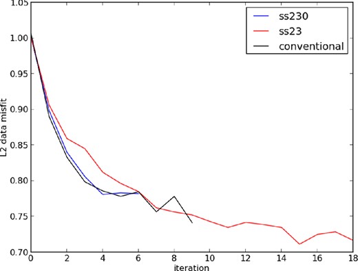
Decrease in data misfit versus iteration for encoding strategies. One conventional iteration is approximately 10 times the cost as one ‘ss230’ iteration, and 100 times the cost as one ‘ss23’ iteration. While ‘ss23’ achieves lower data misfit, the corresponding reconstructed models are more prone to crosstalk noise and crossline aliasing (Figs 10 and 11).
In Fig. 10 we plot the starting model and FWI-derived models for each encoding scheme. Cross-sections in the x–y plane at depths of 237 m (Figs 10a–d) and 1213 m (Figs 10e–h) are shown. In the near-surface, the channel network imaged in Sirgue et al. (2010) and Etienne et al. (2012) is clearly observed, although we differ slightly in the depth coordinate from their models (175 m and 150 m, respectively). Relative to their studies, our model updates are more strongly restricted to the OBC array, evidenced by the lack of illumination of the near-surface channel at position (x, y) = (9.5 km, 9.5 km). Conventional FWI without source encoding (Fig. 10d) slightly improves this illumination. At depth 1213 m we observe the extension of the low-velocity zone (Fig. 10h, yellow arrow), similarly reported by Sirgue et al. (2010) and Etienne et al. (2012) at depths of 1050 m and 1260 m, respectively. Their higher resolution models demonstrate greater perturbation than ours, and interpret this feature as a gas-filled fracture. In Fig. 11 we plot model cross-sections in x–z and y–z plane for models derived with each encoding scheme. While both schemes appear to duplicate similar features (e.g. layered interfaces), crosstalk noise is most notably apparent with the ss23-derived model, as is expected. Little difference is observed between model ss230 and serial-source, conventional FWI.
In Figs 12 and 13 we plot the waveform residuals along a horizontal line of recorded waveforms for a single source (Figs 12a and c) and a supershot of 100 encoded sources (Figs 13a and c), corresponding to initial and final models of Figs 10 and 11. In each case we use the final model derived from ss23. It is apparent that, despite the model improvements as shown in Figs 10 and 11, only a moderate decrease in seismogram misfit is observed. For the single-source case of Fig. 12, misfit is most visibly reduced for shallow reflections in the near-zero offset (time ∼1 s), and subsequent reflections arriving between 2 and 3.5 s. Large-amplitude Scholte waves, induced by the water–solid interface, are not modelled by our acoustic modelling engine and therefore have no misfit reduction (Fig. 12b). Farther-offset traces observe cycle-skipped first arrivals (Fig. 12d).
The same observations hold for the encoded source residuals in Fig. 13, but are less obvious due to the complexity of the blended waveforms. Fig. 13(b) displays a single supershot record, whose encoding contains a nearby shot (compare to neighbouring records Fig. 13a). Misfit is reduced moderately at for the first arriving waveforms at times 0.3–0.5 s, but larger waveforms near time 2.0 s, similar to the expected arrival of a Scholte wave as in Fig. 12(b), are not accounted for. A supershot record consisting of 100 encoded sources from Fig. 13(d), whose nearest source is at comparably farther offset, demonstrates less misfit reduction. However, cycle skipping is less severe as with the single shot record in Fig. 12(d). With 100 encoded sources selected randomly from a set of 2302, we expect that first arrivals from at least one or more sources will be within the cycle-skip regime.
Terminal misfit decrease for encoding schemes ss230 and ss23 was found to be 22 per cent and 29 per cent, respectively (Fig. 14). Interestingly, greater misfit reduction is observed when using greater levels of encoding, although the derived models appear to be of poorer quality. Despite attempting a number of encoding schemes, the misfit reduction over all data space remained in the vicinity of 20 per cent. Attempting iterations with additional depth thresholds, deeper than the initial 1050 m, did not decrease misfit. Poorer model reconstruction and data misfit decrease were observed when inverting for the entire 8 s of data available. Two other strategies (not shown) were considered that yielded only a slight improvement in misfit decrease. In one case we progressively modelled larger time windows (inverting for 1, 2, 4 and 8 s of data, sequentially). In another case we considered batches of encoded sources, where each assembly of 230 encoded supershots was distributed across 10 iterations (rather than one). In both of the cases, however, the marginal improvement in misfit reduction was offset by a substantial increase in number of FWI iterations, thus removing the overall gain of source encoding. We therefore speculate that strategies chosen in the non-linear optimization problem, and not encoding, are more crucial to improving upon the current results.
6 CONCLUSIONS
We have demonstrated the utility of encoded-source FWI in large-scale application to real data. We have presented an FWI workflow that is optimized to iterate over encoded sources, efficiently producing acoustic velocity model updates. Encoded-source FWI generates blended waveforms where conventional inversion and data-processing strategies may not be readily applicable. Therefore, we choose simple, robust strategies that are suitable for simultaneously simulated sources. These include inverting low-frequency bands, and preconditioning the gradient search direction via an absolute threshold given as a function of depth. Whereas conventional FWI tends to rely on scale separation in the data domain by distinguishing differing wave arrivals as a function of time and offset, encoded-source FWI with random source locations simplifies this (for better or worse) by removing the concept of ‘offset’.
Although models derived from encoded-source FWI contain crosstalk artefacts, the potential remains for their exploitation in a seismic processing workflow. In particular, for fixed-spread acquisitions where the modelling cost is independent of source location, encoded sources offer the ability for fast evaluation of the misfit functional and model sensitivities. The computational cost of iterating the Valhall model with 23 encoded supershots, an approach that clearly imaged subsurface channels, was only on the order of a few hundreds of CPU hours. This relatively cheap cost, in addition to the quite general methods of data- and model preconditioning that we have applied, suggests that the presented workflow could be applied in an automated fashion to raw data for immediate results, either for purposes of tomography or quality control.
In a synthetic application, we have demonstrated the ability of encoded-source FWI to finely reconstruct large-scale models in the most extreme case of full-source assembly. Although we do not believe such an optimistic result to be reasonable on real data, the successful demonstration of Figs 3 and 4 does provide a few important results. First, encoded-source FWI offers an extremely cheap means to verify early-stage results of a general FWI workflow. Second, synthetic acoustic FWI on data with the same physical modelling engine, that is, the case of the so-called ‘inversion crime’, is quite robust with respect to crosstalk noise. Although this could be fairly criticized as far too simplistic a scenario in which to draw conclusions on real data (our attempts to invert the Valhall data with a single encoded supershot failed to produce coherent velocity models), the experiment nevertheless yielded results that were valuable for real data application, evidenced by the tomographic images reconstructed by less ambitious encoding schemes (Figs 10 and 11).
There is a well-known trade-off in FWI with respect to noise in low frequencies (and thus large spatial wavelengths) versus starting model quality. Our synthetic studies (Fig. 6) demonstrate a frequency-dependent response of encoded-source FWI concerning this trade-off. Noise degrades the efficiency gain that can be exploited by encoded sources; this was demonstrated in the frequency-domain study of Ben-Hadj-Ali et al. (2011) as need for a greater number of inverted frequencies. In both synthetic and real-data application, we observe an overall efficiency gain (judged by the number of encoded supershots per iteration multiplied by the number of iterations for a given model resolution) favouring heavier levels of source compression. For noise-free synthetics, full-source assembly is the most efficient approach. Although full-source assembly failed to produce an interpretable velocity model on the Valhall field data, partial-source assembly with as few as 23 encoded supershots succeeded. Clearer resolution (in terms of less visible artefacts) was shown with the less-compressed scheme of 230 encoded supershots, but at the expense of greater overall cost.
Despite attempting a number of different encoding strategies on the Valhall data, each in the range of one to two orders of magnitude speedup per FWI iteration, reduction in data misfit remained in the vicinity of 20–30 per cent. We believe that, with the workflow proposed in this study, encoded sources offer an accurate and efficient way to compute the model gradient. Further convergence could be achieved by accurately accounting for anisotropic effects, as well as with more sophisticated strategies to solve the underlying non-linear optimization problem (e.g. utilizing an approximate Hessian). Our approach remains to be demonstrated on high frequencies, however, as we only inverted up to 4 Hz. Still, the results attained demonstrate potential to greatly accelerate the early stages of acoustic velocity inversion on fixed-spread data.
We acknowledge funding from the QUEST (Quantitative Estimation of Earth's Seismic Sources and Structure) consortium, an initial training network funded by the 7th Framework ‘People’ Programme by the European Commission. We are grateful for the efforts of reviewers Vincent Prieux and Yann Capdeville for the time dedicated to review the manuscript. We also thank Vincent Prieux for contributing ideas that improved our final results on the Valhall model. We acknowledge BP for access to the Valhall field data, and Jean Virieux and Olav Barkved for assistance in receiving the data. We thank Jean Virieux and Vincent Etienne for spirited cooperation in this research project. We thank Stéphane Operto for fruitful discussion and assistance in acquiring the overthrust model, and Daniel Peter and Yang Luo for assistance in developing and applying the SPECFEM3D solver for our application. We thank Gerhard Pratt for helpful advice regarding the source wavelet inversion, and Christian Pelties for contributing ideas towards workflow strategies.
This work utilized computing resources on SuperMUC machine (www.lrz.de/services/compute/supermuc), a Peta-scale supercomputer commissioned by the Leibniz Supercomputing Centre (Leibniz-Rechenzentrum; LRZ) near Munich, Germany. We thank the support staff at the LRZ for assistance in adapting our workflow for efficient implementation on SuperMUC.
Now at: Schlumberger WesternGeco, 3750 Briarpark, Houston, TX 77042, USA.
