Increasing the number and signal-to-noise ratio of OBS traces with supervirtual refraction interferometry and free-surface multiples

Abstract

1 INTRODUCTION

Geophysicists use large-offset refraction surveys to image the gross crustal velocity structure of the earth (Musgrave 1967; Mooney & Weaver 1989; Zelt & Smith 1992; Sherif & Geldart 1995; Funck et al.2008), as well as the detailed structure within a few hundred metres of the near surface (Zhu et al.1992). For large-offset surveys the imaging can extend down to the upper part of the mantle (Operto & Charvis 1996) if the source–receiver offsets are sufficiently large.¹ In a wide-offset land refraction survey, the source can be tens to hundreds of kilograms of explosives buried to a depth of 50 m or more, and the seismometers are spaced over a range of up to several hundred kilometres (Mooney & Weaver 1989). The typical receivers are one- to three-component portable recorders that record continuously, sometimes with more than several hundred recording stations per shot. Prior to the test ban treaty, nuclear explosions generated high quality refraction arrivals with recorded diving waves reaching depths of 700 km (Nielsen & Thybo 2003) or more. In one such explosion, the average receiver spacing was 10–15 km over a distance of 3000 km.

For large-offset marine surveys, there are many shots² but typically fewer recording stations. The recording stations can be floating sonobuoys or receivers placed on the seafloor. Seafloor-mounted stations are typically known as ocean bottom seismometers (OBS). These instruments generally record continuously for hours to weeks during the shooting survey, and are later released with an acoustic command to float to the surface for recovery. After clock drift corrections the OBS data are cut into traces corresponding to the source shots. For example, the Kerguelen Plateau survey of Operto & Charvis (1996) deployed five OBS stations evenly spaced over line lengths of up to 160 km with an average shot spacing of about 185 m. Another example is a Nova Scotia marine refraction survey (Funck et al.2004) with 19 OBS stations and a maximum source–receiver offset of 490 km. The source array consists of 12 airguns with a shot spacing of 132 m.

Although used successfully in many areas and environments, a typical limitation of OBS surveys is that the source signal generally becomes weaker with large-offset traces. This means that the far-offset traces often become too noisy for accurate first-arrival picking.

To improve the quality of far-offset OBS data in large-offset refraction surveys, Dong et al. (2006), Bharadwaj & Schuster (2010), Mallinson et al. (2011) and Bharadwaj et al. (2012) developed the theory of refraction interferometry. Here, virtual traces are generated by the summed correlation (Dong et al.2006; Mikesell et al. 2009) of windowed traces to enhance the signal-to-noise ratio (SNR) by a factor of |$\sqrt{N}$|⁠, where N is the number of post-critical sources offset from a specific pair of receivers. In this case, the noise in the traces is assumed to be zero-mean additive white noise. The theory is based on the reciprocity equations of convolution and correlation types, and has been validated on land data from both exploration and engineering surveys. The key assumption is that the enhancement of the SNR in first arrivals is only valid for head waves, not pure diving waves unless the diving waves bottom out at the same depth for more than, say, 4 or more wavelengths. Numerical experiments suggest that interfering head waves within a thin layer also provide the stationary source points for enhancing the SNR of first arrivals.

This paper extends the supervirtual interferometry (SVI) theory of Mallinson et al. (2011) and Bharadwaj et al. (2011) to also incorporate free-surface multiples for enhancing the SNR of refractions as well as to create virtual OBS stations. The refraction arrivals recorded at these virtual OBS stations can more than double the number of traces recorded by the original survey. Doubling the number of recorded refraction arrivals leads to a denser illumination of the subsurface, which can improve the reliability of the resulting refraction tomograms. Here, we demonstrate the effectiveness of the SVI method on refraction data recorded during the TAIGER project, a large, international geophysical survey lead by U.S. and Taiwanese scientists to determine crustal structure around and across Taiwan. The test data are recorded using a 220 km shot line and six evenly spaced OBS stations deployed offshore of Taiwan.

The first section of this paper presents the established theory of refraction interferometry, but also extends it to multiple refractions. These multiple refractions from the free surface effectively create virtual OBS receiver gathers at locations between the original stations as well as locations outside the original receiver array. The second section demonstrates this procedure on both synthetic data and with the Taiwan field data. Finally, the last section summarizes the salient points of our paper.

2 THEORY

The theory of supervirtual refraction interferometry is presented in Bharadwaj & Schuster (2010), Mallinson et al. (2011) and Bharadwaj et al. (2011), so we only illustrate the essentials in Fig. 1. This will then lead to the recipe for creating virtual refraction data from free-surface multiples recorded at a virtual OBS station (see the dashed virtual hydrophone at A^′ in Fig. 3c, located next to the actual OBS station).

Figure 1.

Open in new tabDownload slide

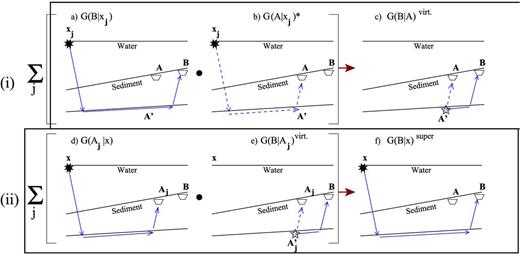
The steps for creating supervirtual refraction arrivals in the case of OBS data. |$\bf A$| and |$\bf B$| are the positions of OBS stations while |$\bf x$| denotes the source position. Dashed ray paths correspond to those with negative traveltimes compared to the positive traveltimes associated with the solid ray paths. (i). Correlation in the time domain of the recorded trace at |$\bf B$| with that at |$\bf A$| gives the virtual trace for different source positions. The summation indicates stacking over source positions x_j as in equation 1 (ii). The supervirtual trace is computed with eq. (2) by convolving in the time domain, the stacked virtual trace G(B|A)^virt. with the actual refraction trace G(A_j|x) and summing over A_j. The open star at A^′ indicates the virtual source position on the refractor.

Assume the acquisition geometry illustrated in Fig. 1 where only head-wave arrivals are generated and recorded by the indicated receivers; the refractor interface can have any smooth geometry, with the underlying homogeneous velocity faster than that of the overlying medium. The trace at location B records a head wave excited by the harmonic source at |$\bf x$| and is mathematically approximated in the frequency domain as |$G({\bf {B}}|{\bf {x}})=\text{e}^{\text{i} \omega \tau _{xB}}=\text{e}^{\text{i} \omega (\tau _{xA^{\prime }}+\tau _{A^{\prime }B})}$|⁠, where the angular frequency variable ω is silent in G(B|x) and geometrical spreading effects are conveniently ignored. Here, τ_xB represents the refraction traveltime along the xA^′B ray path shown in Fig. 1(a). Similarly, the trace recorded at A is given by |$G({\bf {A}}|{\bf {x}})=\text{e}^{\text{i} \omega \tau _{xA}} = \text{e}^{\text{i} \omega (\tau _{xA^{\prime }}+\tau _{A^{\prime }A})}$|⁠, where |$\tau _{xA} = \tau _{xA^{\prime }}+\tau _{A^{\prime }A}$| is the refraction traveltime along the xA^′A ray path in Fig. 1(b).

Enhancing the SNR of primary head waves. The following describes the steps for generating a supervirtual trace (see Bharadwaj et al.2011) at B for a source at x with the SNR enhanced by |$\sqrt{N}$| (Yilmaz 1987), where N is the number of post-critical sources.

• Generate the virtual trace G(B|A)^virt. by summing the spectral product G(B|x)G(A|x)* over the x variable to get

  \begin{eqnarray} Im[G({\bf {B}}|{\bf {A}})^{\rm virt.} ] &\approx & k \sum _{j=1}^{N_{\rm s}} G({\bf {B}}|{\bf {x}}_j)G({\bf {A}}|{\bf {x}}_j)^*, \end{eqnarray}

  (1)

  where k is the wavenumber at the hydrophone, N_s is the number of post-critical source positions for the receiver at B, Im[G] stands for imaginary part of the function G, and the far-field approximation is assumed (Wapenaar & Fokkema 2006). The phases along the common ray paths in Figs 1(a) and (b) cancel in |$G({\bf {B}}|{\bf {x}})G({\bf {A}}|{\bf {x}})^* =\text{e}^{\text{i} \omega (\tau _{xA^{\prime }}+\tau _{A^{\prime }B})} \text{e}^{-\text{i} \omega (\tau _{xA^{\prime }}+\tau _{A^{\prime }A})}= \text{e}^{\text{i}\omega (\tau _{A^{\prime }B}-\tau _{A^{\prime }A})}$| to give the virtual head wave G(B|A)^virt. illustrated by the ray diagram in Fig. 1(c). The kinematics of this diagram suggests that the virtual head-wave arrival recorded at B can be excited by N_s different source positions at x, so stacking G(B|A)^virt. over x increases the SNR of the head wave by |$\sqrt{N_{\rm s}}$| (Dong et al.2006).

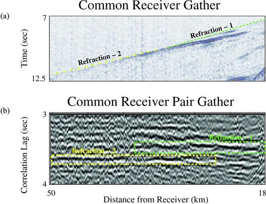
   To distinguish head waves from diving waves, Dong et al. (2006) defined the common receiver pair gather (CPG), shown in Fig. 2(i), as a collection of virtual traces |$g({\bf {B}},t|{\bf {A}},0)^{\rm virt.}={\mathcal {F}}^{-1}[G({\bf {B}}|{\bf {A}})^{\rm virt.}] = {\mathcal {F}}^{-1}[G({\bf {A}}|{\bf {x}}_j)^* G({\bf {B}}|{\bf {x}}_j)]$| plotted against different post-critical source positions at x_j. In this case A and B are fixed hydrophone positions that are post-critically offset from the sources at x1, x2 and x3. They showed that if the events in a CPG are flat (i.e. they occur at the same time) then such events originate from true head waves that propagate along the same refractor; otherwise they are likely to be a pure diving wave or an event that does not satisfy the implicit assumption of a head wave travelling along a vertical slice of the earth. The CPG traces can be used to test whether the first arrivals are head waves from the same refractor or not. Their variations in time and amplitude can also be used to examine the lithological nature of the refracting boundary (Dong et al.2006).

• Compute the spectral product G(A|x)G(B|A)^virt. and sum over N_g post-critical hydrophone positions A to get the supervirtual trace (Bharadwaj et al.2011; Mallinson et al.2011):

  \begin{eqnarray} G({\bf {B}}|{\bf {x}})^{\rm super} &=& 2ik \sum _{j=1}^{N_g} G({\bf {A}}_j|{\bf {x}}) G({\bf {B}}|{\bf {A}}_j)^{\rm virt.}. \end{eqnarray}

  (2)

  The ray diagrams for the above equation are illustrated in Figs 1(d) and (e) and show that the negative phase for the A^′A path in (e) cancels the positive phase along A^′A in (d) to give the head-wave ray path in (f).

Figure 2.

Open in new tabDownload slide

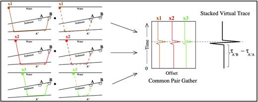
Here, |$\bf A$| and |$\bf B$| are the positions of OBS stations while |$\bf x1$|⁠, |$\bf x2$| and |$\bf x3$| are the source positions. Head-wave arrivals from different source positions become aligned in a CPG after cross-correlation; these aligned arrivals can be stacked to increase the head-wave signal strength.

Sometimes even supervirtual refractions are of insufficient SNR or the station density is too low, so we need to improve the quality and quantity of the data. One such opportunity is to elevate the status of coherent noise, namely free-surface multiples, to be signal.

Creating virtual OBS stations from refraction multiples. Fig. 3 illustrates that the trace at A with a free-surface refraction multiple can be transformed into a virtual trace at A^′ containing a primary refraction; the dashed hydrophone at A^′ is denoted as the virtual hydrophone. The ray path between A and A^′ can be computed by ray tracing if the water-bottom topography is known and the angle of incidence of the refraction arrival is computed from the components recorded by the OBS station. An alternative is to consider that the virtual hydrophone is located at the mirror image point, denoted by the red hydrophone in Fig. 3(a); in this case, rays are traced from the original source position to the mirror hydrophone. A time shift can then be calculated and applied to transform the refraction multiples into refraction primaries virtually recorded at virtual seafloor hydrophones located next to the actual hydrophones.³ In fact, if refraction multiples up to the Pth order have high SNR then this means that the original survey can theoretically increase the number of OBS stations by a factor of P. These extra glimpses of the subsurface can provide a more comprehensive imaging of the subsurface by refraction tomography and migration. The next section presents the equations for enhancing the SNR of refraction arrivals by applying the SVI method to refraction multiples.

Figure 3.

Open in new tabDownload slide

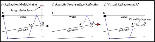
(a) Trace with a refraction multiple recorded at A correlated in the time domain with a (b) trace associated with the free-surface reflection (here, the dashed ray path indicates negative traveltime) yields the (c) virtual trace with the primary refraction at A^′. This is the procedure for transforming a first-order refraction multiple recorded at A into a primary refraction recorded at A^′, the virtual receiver location.

Enhancing the SNR of refraction multiples and their transformation to primaries. Refraction multiples are often noisier than their primaries and so their SNR should be enhanced prior to transformation into primaries at virtual hydrophone locations. Towards this end we propose the application of a modified supervirtual method to the multiples. This procedure is illustrated in Fig. 4 and is described in the following steps.

• Creating virtual refractions from multiple refractions. Denote the trace with the first-order free-surface multiple as |$\tilde{G}({\bf {A}}|{\bf {x}})$|⁠; in practice, we window about the free-surface multiples in the original records so that much of the primary reflection/refraction energy is extinguished. Form the spectral product |$G({\bf {B}}|{\bf {x}}) \tilde{G}({\bf {A}}|{\bf {x}})^*$| and sum over different x positions that are post-critically offset from the receivers A and B to get the virtual head wave recorded at B

  \begin{eqnarray} Im [G({\bf {B}}|{\bf {A}})^{\rm virt.}] &=& k \sum _{j=1}^{N_{\rm s}} G({\bf {B}}|{\bf {x}}_j) \tilde{G}({\bf {A}}|{\bf {x}}_j)^*, \end{eqnarray}

  (3)

  where N_s is the number of sources post-critically offset from a specified pair of receivers. In this case the virtual head wave associated with Fig. 4(c) can be interpreted as being excited by a virtual source located at A^′′ and its excitation time advanced by the traveltime along the dashed ray; the summation over the N_s source locations enhances the SNR by a factor proportional to |$\sqrt{N_{\rm s}}$| for additive white noise.
• Creating supervirtual primary refractions from G(B|A)^virt.. Supervirtual primaries can be created from multiples and virtual refractions, as illustrated in Figs 4(d)–(f). Here, the trace |${\mathcal {F}}^{-1}[ \tilde{G}({\bf {A}}|{\bf {x}}) ]$| with a windowed multiple refraction recorded at A is convolved in the time domain with the virtual trace |${\mathcal {F}}^{-1}[ G({\bf {B}}|{\bf {A}})^{\rm virt.}]$| to give the supervirtual primary trace |${\mathcal {F}}^{-1}[G({\bf {B}}|{\bf {x}})^{\rm super}]$| as illustrated in Figs 4(f) and mathematically described by the frequency-domain formula

  \begin{eqnarray} G({\bf {B}}|{\bf {x}})^{\rm super} &=& 2i k\sum _{j=1}^{N_g} G({\bf {B}}|{\bf {A}}_j)^{\rm virt.} \tilde{G}({\bf {A}}_j|{\bf {x}}). \end{eqnarray}

  (4)

  The SNR of the virtual trace G(B|A)^virt. is enhanced by |$\sqrt{N_{\rm s}}$|⁠, but the supervirtual primary G(B|x)^super is further enhanced by the multiplicative factor |$\sqrt{N_g}$| if the raw traces G(B|A) have no noise, an unrealistic assumption. It is more realistic to assume that the SNR of the supervirtual primary is only enhanced by the factor |$\min (\sqrt{N_g},\sqrt{N_{\rm s}})$|⁠. However, limited experiments in applying the SVI method to land data (personal communication with Ola AlHagan) suggest that replacing the input data trace with a SVI trace (after one or several iterations of the SVI method) can sometimes greatly enhance the SNR of noisy traces.
• Creating supervirtual multiple refractions from G(B|A)^virt.. Supervirtual multiples with an enhanced SNR can be created from the raw data and the virtual data G(B|A)^virt. using the strategy illustrated in Figs 4(g)–(i) and the following formula:

  \begin{eqnarray} \tilde{G}({\bf {A}}|{\bf {x}})^{\rm super} &=& 2\text{i}k \sum _{j=1}^{N_g} G({\bf {B}}_j|{\bf {A}})^{*{\rm virt.}} G({\bf {B}}_j|{\bf {x}}), \end{eqnarray}

  (5)

  where N_g is the number of hydrophones post critically offset from the source. In the time domain, the above operation is a summation of convolved traces. This enhanced multiple can be considered as being recorded by an mirror hydrophone (red colour) as shown in Fig. 3(a). Furthermore, this refraction multiple record can be cross correlated with the analytic free-surface reflection within the water layer to get the virtual OBS trace with the ray diagram shown in Fig. 3.

Figure 4.

Open in new tabDownload slide

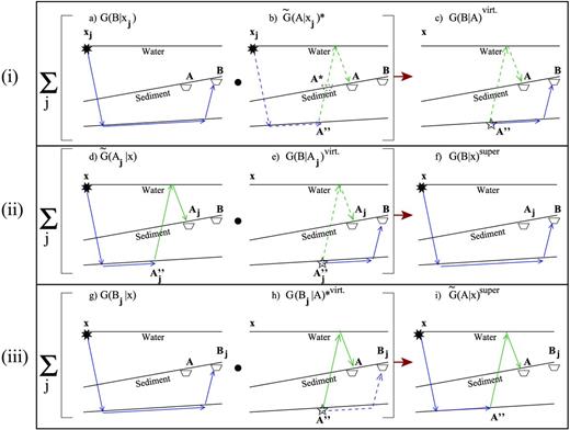
Diagrams illustrating the supervirtual interferometry procedure. Note that the refraction multiple recorded at B instead of at A can also be used in the above method. In this figure the dashed ray paths correspond to those with negative phase. (i) Cross-correlation in the time domain and summation over j for different source positions x_j yields a stacked virtual trace. (ii) Virtual trace generated in (i) is convolved with the recorded refraction multiple to get a supervirtual refraction primary at B. (iii) Cross-correlation of virtual trace generated in (i) with refraction primary to get a supervirtual refraction multiple at A.

In summary, the supervirtual refraction interferometry method can be used to create enhanced traces |$\tilde{G}({\bf {A}}|{\bf {x}})^{\rm super}$| in eq. (5) that, in principle, can be used to better illuminate the subsurface and increase the SNR of the head-wave arrivals.

3 SYNTHETIC AND FIELD DATA RESULTS

Tests on synthetic data and field data from an OBS survey will now be used to illustrate the benefits and pitfalls of supervirtual refraction interferometry applied to both primary refractions and those related to free-surface multiples.

3.1 Synthetic SVI data results

The common receiver gathers (CRGs) for an OBS experiment are simulated by a finite-difference solution to the 2-D wave equation for the acoustic velocity model in Fig. 5. The peak frequency of the source wavelet is 6 Hz. There are ten receiver gathers spaced at 6 km intervals and the source spacing of 45 m is used to generate 1600 traces per receiver gather. The OBS stations are on the sea floor at a depth of 3000 m, the traces simulate pressure field measurements and a computed OBS gather is shown in Fig. 6.

Figure 5.

Open in new tabDownload slide

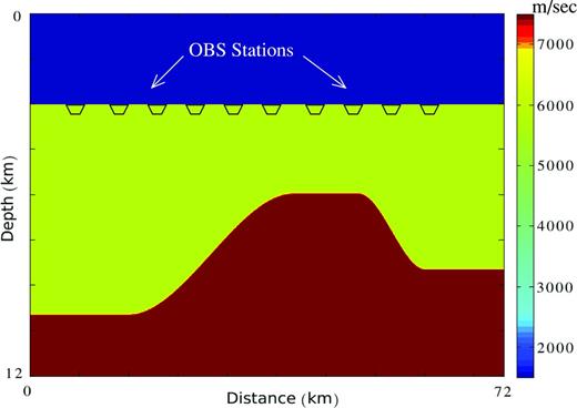
Crustal model where the OBS receivers are along the ocean floor at the depth of 3 km (as marked) and the sources are near the free surface.

Figure 6.

Open in new tabDownload slide

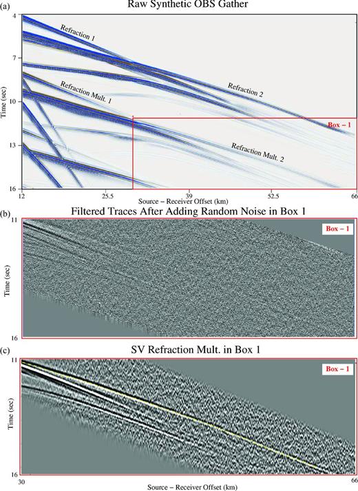
(a) Synthetic OBS gather of the first station marked in the Fig. 5 velocity model. (b) Zoomed view of band-pass filtered traces in Box-1 after adding random noise. (c) Supervirtual refraction multiple with enhanced SNR compared to traces in (b).

Fig. 6(b) shows a synthetic OBS gather (approximately windowed around the first-order refraction multiple) after adding random noise. Fig. 6(c) depicts the corresponding supervirtual receiver gather with an enhanced SNR for the 1st-order refraction multiple. In this case, approximately N_s = 250 traces are used in the stacking process for a theoretical SNR enhancement of 15.8. The enhanced SNR improvement here is similar to that in Bharadwaj et al. (2011), except free-surface refraction multiples are enhanced rather than primary refractions.

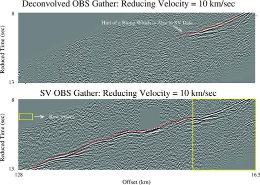
Traveltime tomography results. First-arrival traveltimes are picked from the traces generated for the Fig. 5 model and inverted by a traveltime tomography algorithm (Nemeth et al.1997). This test is designed to illustrate some of the benefits in incorporating extra traveltimes from multiple refractions into a traveltime tomography algorithm. The source–receiver geometry is that of an OBS marine experiment where the shot interval near the free surface is 45 m, and there are 16 OBS receivers on the sea floor with a receiver spacing of 4000 m. The acoustic shot gathers are generated by an |$O(\text{d}t^2, \text{d}x^4)$| finite-difference solution to the 2-D acoustic wave equation with a Ricker source wavelet peaked at 5 Hz. A total of 16 receiver gathers are generated and the first-arrivals are picked to give a total of 25 616 traveltimes. The data also contain free-surface related multiples so that after separation, extra refraction times can be picked from the 1st-order multiples. Random noise was added to the synthetic data so that only 75 per cent of the traveltimes could be accurately picked by a human interpreter.

The traveltime matrix for these picked times is illustrated in Fig. 7(i) and used as input into a traveltime tomography algorithm (Nemeth et al.1997). The resulting tomogram shown in Fig. 7(ii) shows a poor resolution of the Moho boundary as well as many artefacts due to the sparse ray coverage, illustrated in Fig. 7(iii). The noisy traces were then input into the SVI algorithm and the resulting first arrival traveltimes can now all be reliably picked as shown by the traveltime matrix in Fig. 7(iv). The associated velocity tomogram in Fig. 7(v) shows fewer artefacts than seen in Fig. 7(ii), but there is still a limited resolution of the Moho boundary. The ray diagram in Fig. 7(vi) suggests this is due to sparse ray coverage in some areas of the model. To densify the ray coverage, the first-order multiples picked from the SVI data set are transformed into virtual primary refractions at virtual OBS receivers. These picks are shown in the Fig. 7(vii) traveltime matrix. The resulting tomogram in Fig. 7(viii) shows reduced artefacts compared to Fig. 7(v). The left and right flanks of the bump are more accurately imaged than in Figs 7(v) or (ii). However, the top of the bump in Fig. 7(viii) appears to be slightly less accurate than that in Fig. 7(v). This might be because the associated rays, as seen in the ray density plot, are not pure head waves. This is a problem that could be possibly avoided by only admitting flat events in a common pair gather. Overall, this result illustrates some limited benefits of incorporating traveltimes from SVI primaries and multiples into a tomography algorithm. It also suggests that one should only use virtual traveltimes associated with flat events in the common pair gathers.

Figure 7.

Open in new tabDownload slide

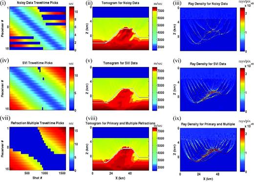
(i) Traveltime matrix in the case where the first arrivals in some of the synthetic traces cannot be picked because they have low SNR. (ii) Tomogram generated using noisy data traveltime picks. The solid grey lines denotes the actual MOHO boundary for comparison. (iii) Ray density plot corresponding to the noisy data case. The second row of plots is the same as the first row, except the input data are the SVI traveltime picks for the primary refractions. The third row is the same except the input data are the traveltimes for the 1st-order multiple refraction traveltimes picked from the supervirtual refraction traces. The tomogram in (viii) is computed using both the primary and 1st-order multiple refraction travel times in the SVI data.

This example illustrates a potential liability of this method: long-offset refraction arrivals extracted from the SVI records might not necessarily originate from deeper refraction interfaces. Almost every portion of the synthetic Moho interface could have been probed by refraction arrivals with intermediate offsets between the source and receiver, so that the long-offset traveltimes supplied redundant information about the Moho. The value of redundancy in this case, is that the increased ray density reduces artefacts in the tomogram. This suggests that the long-offset SVI traveltimes extracted from a wide-offset refraction survey might be associated with later-arrival head waves from the Moho, and not first-arrival refractions from the mantle.

3.2 Taiwan OBS data results

Six OBS gathers from the TAIGER field survey near Taiwan were recorded by a team of scientists lead by the University of Texas at Austin and National Taiwan Ocean University (Keelung, Taiwan). Here, the inline OBS station spacing is 15 km and the inline shots are spaced at 150 m intervals. The total number of shots is 1516 and the maximum source–receiver offset is 181 km. Fig. 8(a) shows a recorded CRG along with the positions of other stations [marked (ii) to (vi)] in the survey. The recording time of the traces is 30 s.

Figure 8.

Open in new tabDownload slide

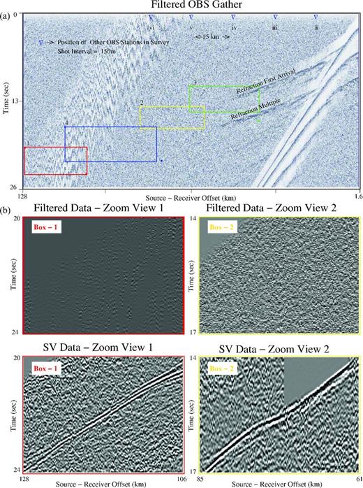
(a) A filtered OBS gather, where both the first arrivals and the refraction multiples are visible only up to a limited offset. The positions of other OBS stations in the survey are marked as well, which are separated from one another by approximately 15 km. (b) Zoomed views at corresponding coloured boxes (1 and 2 in a) of both filtered and supervirtual data. The raw data have been muted prior to SVI processing such that the refraction arrivals from other shallow refractors are removed. The zone with no data in the lower right box is a result of muting.

Fig. 9 shows a CPG for the OBS station pair (v) and (vi) marked in Fig. 8(a). Fig. 10(b) shows a common pair gather where one of the receivers is an mirror hydrophone that virtually records⁴ the first-order refraction multiple (cross-correlation step shown in Fig. 4i). It can be concluded from the horizontal events in the CPG that the first-arrivals are mostly refracting along the interface as head waves. All the traces in Fig. 9 can be summed together to get a stacked virtual trace with an enhanced SNR.

Figure 9.

Open in new tabDownload slide

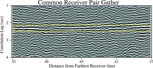
This plot shows a common pair gather generated for different source positions as in Fig. 2. The correlation lag on the vertical axis is equal to the propagation time with an unknown excitation for waves to propagate from the virtual source on the refractor to one of the receivers in the receiver pair. The position of the two OBS stations for this gather is marked as (v) and (vi) in Fig. 8(a).

Figure 10.

Open in new tabDownload slide

(a) A common receiver gather from the Taiwan OBS data set corresponding to the station (vi) as marked in the Fig. 8(a). (b) A CPG formed by correlating the refraction primaries with the first-order refraction multiples recorded at this receiver for different source positions near the sea surface. Both primary and multiple refractions are separated from the OBS traces by applying time windows. The procedure is illustrated in Fig. 4(i) except the positions of the two stations (marked A and B) coincide with one another. The CPG suggests the presence of refraction arrivals from two different refractors marked by green and yellow boxes.

Using the work-flow described below, supervirtual traces are created from the six Taiwan CRGs, to give the results shown in Figs 8, 11, 12 and 13. Fig. 11 compares the supervirtual refraction traces in Box-3 and Box-4 of Fig. 8(a) before and after using SVI gathers from first-order multiples during the final stacking (as illustrated in Fig. 4). Fig. 12(b) shows an OBS gather with a first-order multiple, and the enhanced SVI primary and multiple traces are shown in the boxes below. Fig. 13 compares the final SVI traces to the filtered and deconvolved traces and reveals that more than thrice the number of traces can be reliably picked in the SVI gather.

Figure 11.

Open in new tabDownload slide

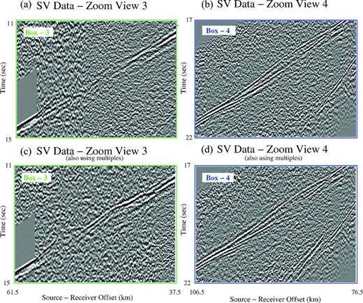
(a) Supervirtual traces in boxes 3 and 4 of Fig. 8(a) without using multiples. (b) Traces corresponding to (a) after stacking supervirtual traces with primary and first-order multiples.

Figure 12.

Open in new tabDownload slide

(a) The record at the OBS station [marked (iii) in Fig. 8(a)]. (b) Zoomed view of both filtered and supervirtual refraction primary traces in the Box-1 (yellow). (c) Zoomed view of filtered and supervirtual refraction multiples in the Box-2 (cyan).

Figure 13.

Open in new tabDownload slide

(a) Raw OBS and (b) SVI gathers from Fig. 8(a) after windowing around the first arrivals. Both primaries and multiples are used for the generation of the SVI traces.

3.2.1 SVI interferometry processing work flow

The flowcharts in Fig. 14 depict the processing steps for obtaining supervirtual traces, and the details are described below. Since the recorded refraction multiples can be considered to be arrivals recorded at mirror hydrophones, the processing steps are the same as those for primary refraction arrivals.

• Pre processing: Carefully window around the first arrivals and refraction multiples associated with a particular refractor in each OBS gather. The window length is 1.75 s in our tests with the Taiwan data. A 1-3 Hz high-pass filter is used to help remove low-frequency noise. To deconvolve the raw data, a prediction-error filter (filter length = 48 samples or 0.24 s in length) is used (Peacock & Treitel 1969) with a prediction lag of 0.032 s and 1 per cent damping.

• Generating a stacked virtual trace: Generate virtual traces by cross correlation of traces recorded by a pair of seismometers as in Fig. 1(i) where primaries are used, or as in Fig. 4(i) where refraction multiples are used. Stack over their common source positions x_j after muting the traces with strong noise (similar to the shot noise in Box-1 of Fig. 8a). The result is a stacked virtual trace whose SNR is improved. The position of x should be selected such that it is post-critically offset from the station pair at A and B and the windowed refraction arrivals are from the same refractor. Approximately 150 such virtual traces can be stacked in the present data set to give, ideally, a |$\sqrt{150} \approx 12$| enhancement of SNR.

• Convolution: Window around the dominant refraction corresponding to the virtual travel time in the virtual trace. Note that this arrival should be at the same travel time regardless of the virtual traces selected from the CPG to stack. This ensures that the traveltime for this event corresponds to the virtual traveltime for head waves to propagate between the two OBS stations. The windowed version of the stacked virtual trace can be used to convolve with the corresponding recorded traces to get the supervirtual traces. In general there are two possible approaches to compute a supervirtual trace from a virtual trace. Approach 1 is to follow Dong et al. (2006) and pick the first arrival time τ_Bx in the raw trace for a source at x; this trace is assumed to have a high SNR so the time is picked with acceptable accuracy. The τ_Bx can be used to find the time shift Δτ to time shift the virtual refraction at B so that it arrives at the actual traveltime τ_Bx, that is, Δτ = τ_Bx − τ^virt._xB − τ^virt._Ax. This value of Δτ can then be used to time shift every virtual trace associated with the receiver pairs A − B for increasing values of the B index. This time shifting is kinematically equivalent to the convolution step in Fig. 1(ii) and Figs 4(ii)–(iii), except that it does not introduce extra noise by convolving noisy traces with clean ones. Alternatively, the other approach is that a windowed version of a stacked virtual trace can be used to convolve with the recorded trace. The second approach is what we used to compute supervirtual traces; this was possible because some of the raw traces had a high SNR.

• SVI traces: All of the above steps can be repeated for different receiver positions |$\bf A$| to generate N_g supervirtual traces, which can then be stacked together to enhance the SNR by |$\sqrt{N_g}$|⁠. Since the number of OBS stations is small in our field data example, we effectively obtained a SNR enhancement due to convolution of windowed and stacked virtual traces with the corresponding recorded traces of high SNR. Also, only a time shift correction was sometimes applied to the raw traces rather than convolution. After stacking, the prediction-error filter as in (i) is applied to the stacked SVI traces followed by a bandpass filter to display the final results.

Figure 14.

Open in new tabDownload slide

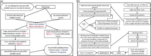
Flowcharts for processing the Taiwan OBS data. (a) An overview. (b) Steps for creating supervirtual receiver gathers.

3.2.2 Reliability tests for SVI data

Finally, reliability tests must be performed to insure that the supervirtual events are not artefacts created by processing. Our suggested reliability tests are the following:

• Test 1: Perform simulations on synthetic data for a model that roughly resembles the actual crustal model and acquisition geometry. For the Taiwan data test, simulations were carried out for the Fig. 5(b) model that roughly approximated the Taiwan source–receiver geometry and a Moho model with a bumpy boundary. The results in Fig. 6 validated the accuracy of the SVI refractions. It is also important to test the sensitivity of the SVI method to enhancing first arrivals associated with diving waves, not necessarily head waves. If the diving wave rays are nearly horizontal for, say five or more wavelengths, then the SVI method will enhance their SNR. This enhancement can be tested by examining the common pair gathers obtained from synthetic seismograms. It might also be possible to apply a time-shift correction to the CPGs to flatten the diving wave events prior to stacking.

• Test 2: Form CPG gathers from the supervirtual data to test for ‘flatness’. If the events are horizontal in this domain, for example, see Fig. 9, then the data satisfy the crucial head-wave assumption.

• Test 3: Compare the moveout curves of the supervirtual refractions generated from primaries to those generated by multiples; test for agreement. Fig. 11 depicts this comparison for the Taiwan data.

• Test 4: Pick traveltimes from filtered records and compare them to those picked from the supervirtual gathers. As shown in Fig. 15(b) the supervirtual and actual travel times⁵ of refraction arrivals mostly agree within T/4 (T ≈ 0.166 s), where T is the dominant period. For field data, we conservatively estimate a picking error to be about T/4, although the actual picking error can be less.

• Test 5: For the Taiwan OBS data set we were able to perform perhaps the most critical and promising test of the SVI method for the OBS data. Several of the profiles had been shot two times-once at a 50 m shot spacing for optimum seismic reflection data and again at 150 or 125 m for the best OBS results. The longer shot spacing for this OBS data shows the previous shot noise (as in Fig. 16a) to be extant mostly at large offset, typically at 90 km with shots at a 60 s interval. The main disadvantage of this approach is the large expense of repeating the shooting and the fact that there is reduced data density. Here we compare SVI data produced from records acquired at a 50 m shot spacing with data recorded by the same instrument shot at a 125 m spacing. As seen in Fig. 16(c), the SVI traces are positioned correctly and the first arrivals are more coherent than those from the 125-m-shot OBS gather. This direct comparison confirms that the SVI method produces consistent results from different surveys, but it also indicates that in many cases excellent OBS data for first-arrival tomography may be acquired that can also be used with multichannel reflection data.

Figure 15.

Open in new tabDownload slide

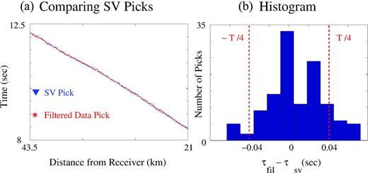
Test 4. (a) Plot comparing first arrival picks from the filtered and supervirtual traces of the OBS gather shown in Fig. 8(a). (b) Histogram plotted after calculating the traveltime differences between the filtered and supervirtual traces in (a).

Figure 16.

Open in new tabDownload slide

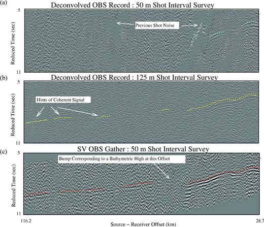
Test 6. (a) OBS gather from a 2-D survey line near Taiwan with a 50-m-shot interval spacing (for optimum seismic reflection data) plotted in reduced time (reducing velocity = 10 km s⁻¹) and windowed around the first-arrival refraction. (b) The gather corresponding to (a) but recorded with a 125 m shot interval spacing so that refractions can be recorded free from the previous shot noise. (c) Supervirtual gather corresponding to (a) which passed the sanity test when compared to the filtered data in (b).

Passing these tests is not a guarantee that the supervirtual refractions are unpolluted by artefacts, but they significantly reduce the chances for false results. Our Taiwan data results passed all of the above tests.

4 CONCLUSIONS AND DISCUSSION

SVI is developed so that free-surface related multiple refractions can also be used to enhance the SNR of primary refraction events by a factor proportional to |$\min (\sqrt{N}_{\rm s},\sqrt{N}_g)$|⁠, where N_s is the number of post-critical sources for a particular refractor and N_g is the number of related hydrophones. This assumes that the SNR of both the primaries and the usable multiples are nearly the same. We also show that refraction multiples can be transformed into primary refraction events recorded at virtual hydrophones located between the actual hydrophones. Thus, data recorded by a coarse sampling of OBS stations can be transformed, in principle, into a virtual survey with P times more OBS stations, where P is the highest order of the usable free-surface related multiple refractions. The key assumption is that the refraction arrivals are those of head waves, not pure diving waves. The effectiveness of this method is validated with both synthetic OBS data and long-offset OBS data recorded offshore from Taiwan. Free-surface multiples were utilized to enhance the SNR of primary refractions as well as to create new virtual OBS records. Results with the Taiwan data show the successful reconstruction of far-offset traces out to a source–receiver offset of 120 km. The supervirtual traces increase the number of pickable first arrivals of primaries from approximately 1600 to more than 3100 for a subset of the OBS data set where the source is only on one side of the recording stations. In addition, the head waves associated with the first-order free-surface refraction multiples allow for the creation of six new CRGs recorded at virtual OBS station located between the actual OBS stations. This doubles the number of OBS stations compared to the original survey and increases the total number of pickable traces from 1600 to 6200.

In summary, we believe SVI opens up new opportunities for long-offset refraction surveys. Compared to the standard processing of OBS refraction data, refraction interferometry can sometimes more than triple the amount of usable data, increase the source–receiver offsets, fill in the receiver line with a denser distribution of OBS stations, and provide more reliable picking of first arrivals. We also believe this method could be used to enhance the SNR of earthquake records where diffraction or refraction arrivals have low SNR. A potential liability of this method is that the long-offset refraction arrivals extracted from the SVI records might not necessarily be the first-arrival refractions, but refractions that arrived after the earlier arrivals from deeper refractors. These deeper refractions might have much weaker SNR and so might be undetectable with the SVI processing. As shown in the synthetic example, the long-offset arrivals were from the Moho, not a deeper interface in the mantle. Nevertheless, this redundancy in the refractor illumination reduces artefacts in the velocity tomogram.

We thank the KAUST Supercomputing Lab for the computer cyclesthey donated to this project. We are especially grateful for the use of the SHAHEEN supercomputer. We also acknowledge the support of the CSIM sponsors (http://csim.kaust.edu.sa).

REFERENCES