


Abstract
Predicting the magnitude and nature of changes in a species’ range is becoming ever more important as an increasing number of species are faced with habitat changes or are introduced to areas outside of the species’ native range. An organism’s investment in life-history traits is expected to change during range shifts or range expansion because populations encounter new ecological conditions. While simulation studies predict that dispersal and reproductive allocation should increase at the range edge, we suggest that reproductive allocation might decrease at the range edge due to energy allocation trade-offs. We studied the reproductive investment of an invasive amphibian, Xenopus laevis, and measured reproductive allocation in three clusters of populations distributed from the centre to the edge of the colonized range of X. laevis in France. Resource allocation was estimated with the scaled mass index of gonads of both sexes during the local period of reproduction of the species. The level of resources allocated to reproduction was lower at the periphery of the colonized range compared to the centre and may be the result of changes in trade-offs between life-history traits. Such a pattern could be explained by interspecific competition or enhanced investment in dispersal capacity.
INTRODUCTION
Shifts in the distribution of a species occur when range edges track environmental changes, when propagules settle beyond an ecological barrier after a discrete introduction event or when evolutionary processes modify the species’ niche and render novel environmental conditions suitable. This issue has been paid renewed attention because of the increasing awareness about the scale of global changes (Parmesan & Yohe, 2003), including human activities that translocate individuals to new areas (Channell & Lomolino, 2000). In this regard, the massive increase in global transport and trade is believed to be responsible for the fast rise in the number of invasive species at the global scale (Lockwood, Hoopes & Marchetti, 2013; Herrel & van der Meijden, 2014). Analysing the process of range expansion is critical to understand and predict the dynamics of a species. This knowledge is also important to guide the management of practitioners who seek to enhance the expansion of reintroduced populations or limit the spread of unwanted aliens (e.g. Roman & Darling, 2007; Shine, 2012; Brown, Kelehear & Shine, 2013).
Range expansion typically occurs after the introduction and settlement of a propagule in a novel environment. It is largely driven by population growth, dispersal and density dependence (Fisher, 1937; Skellam, 1951; Burton, Phillips & Travis, 2010). These parameters summarize the trade-offs in the life-history traits that influence the probability for an individual to reproduce, disperse and survive (Burton et al., 2010). Simulation and empirical studies have demonstrated that allocation of resources to dispersal at the range edge is enhanced during range expansions (e.g. Thomas et al., 2001; Travis & Dytham, 2002; Hughes, Hill & Dytham, 2003; Simmons & Thomas, 2004; Phillips et al., 2008; Léotard et al., 2009; Phillips, Brown & Shine, 2010; Barton et al., 2012; Henry, Bocedi & Travis, 2013; Hudson, Brown & Shine, 2016). Changing dispersal allocation affects the trade-offs with other life-history traits that also require energy or resources (Ferriere & Le Galliard, 2001). Furthermore, Burton et al. (2010) predicted that dispersal and reproductive allocation should increase, whereas resource allocation to competitive ability should be reduced at the range edge. The rationale is that long dispersers have a higher probability to reach a new suitable location at the edge where density-dependent responses and intra-specific competition are low (Brown et al., 2013). At the range core, dispersers would mostly reach already colonized areas (Baguette & Van Dyck, 2007) so that in core areas selection should favour individuals with a high competitive ability (Burton et al., 2010). In contrast with these predictions, the association of high dispersal capacity and low reproduction has been observed (Hughes et al., 2003). It is therefore important to test whether resource allocation to reproduction is reduced or increased at the range edge of expanding populations.
We studied the allocation of resources to reproduction in an expanding population of the African clawed frog, Xenopus laevis (Daudin, 1802) (Anura: Pipidae) in Western France, where it has been introduced. This species has been used worldwide in laboratories for pregnancy tests and as a model in developmental biology and anatomy (Weldon, De Villiers & Du Preez, 2007; van Sittert & Measey, 2016). It has been intentionally or unintentionally introduced in several countries across the world where it is considered as invasive (Measey et al., 2012). A study based on species distribution models suggests that the expansion of the French population is likely to be important during the next decades (Ihlow et al., 2016). In another recent study, an increased allocation to dispersal has been suggested through the observation of an increase in hind limb morphology and stamina at the range edge of the same population (Louppe, Courant & Herrel, 2017). Thus, we hypothesize that at the range edge individuals will allocate fewer resources to reproduction than at the range core. We test this hypothesis by estimating the relative mass of the reproductive organ of males and females with a body condition index.
MATERIAL AND METHODS
Study area and sampling
The African clawed frog was introduced in Western France during the late 1980s, and its estimated colonized area was 207 km2 in 2012 (Measey et al., 2012). Contrary to the Mediterranean-like climate of its native range, the population introduced in France occupies an area where the climate is defined as oceanic altered (Joly et al., 2010), with a relatively high annual mean temperature (12.5 °C), and cumulated annual precipitations reaching 800–900 mm, mainly during winter (Joly et al., 2010). We sampled ponds with an area of less than 500 m2 and a maximum depth between 1 and 3 m. Frogs were captured with fykes (60-cm length × 30-cm width × 6-mm mesh diameter). Capture effort was fixed at 1 trap/50 m2 of water, with a distribution of traps as regular as possible inside the pond, during three consecutive nights, and without repeating this process more than once in the same pond. Every morning, individuals captured in fykes were euthanized with a lethal injection of sodium pentobarbital and dissected just after death. The research permit and the authorization for killing invasive frogs were provided by the Préfet of the Deux-Sèvres department.
D etermination of the optimal period to study reproduction
In California, the period of reproduction of X. laevis occurs from January to November, with a 2- to 3-month peak during spring (McCoid & Fritts, 1989). For the French population, the optimal time frame to estimate reproductive allocation was determined by sampling the gonad mass and the proportion of gravid females from March to October 2014 (no individuals were caught during trapping sessions from November to February). We captured and analysed a total of 408 female frogs to determine the breeding period of this population, with monthly captures in six ponds from the range edge, core and intermediate areas (two in each area), except in October when only two successful capture occurred at the range core and the intermediate area. New ponds were used every month. The optimal time frame was then defined as the period when the proportion of gravid females and the relative mass of reproductive organs [estimated with the scaled mass index (SMI), see below] was increasing and when the females are most likely to start breeding and have to laid many eggs. We then could assess the spatial variation of allocation to reproduction on the next spring, in 2015.
Estimation of the resource allocation to reproduction
The present study was carried out on three clusters of five ponds each, distributed across a part of the colonized range (Fig. 1). The clusters were located at the core area close to the introduction site of the population, the range edge (18 km from the introduction site) and in an intermediate zone between both areas (11 km from the introduction site), respectively. The time since colonization at the centre of the range is close to 30 years (Fouquet, 2001). At the range edge, the study sites were colonized less than 3 years ago, according to local landscape managers and unpublished data. This area was selected because it was the most accurately identified colonization axis during our field studies and because no barrier for dispersion was identified in the landscape. In 2015, 731 frogs were captured to study the resource allocation to reproduction, with a three ponds per week frequency (one pond in each cluster). We captured 82, 102 and 120 females at the range core, the intermediate area and the range edge, respectively. For males, 186, 103 and 138 individuals were captured at the range core, the intermediate area and the range edge, respectively. Data sampling for the reproductive allocation study occurred from 4 April 2015 to 13 May 2015.
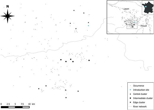
Location of the three pond clusters of Xenopus laevis sampled to analyse the variation in resource allocation to reproduction. Occurrence data for X. laevis were provided by the Société Herpétologique de France.
Morphological and anatomical measures
Individuals were measured and sexed before dissection during 2014 and 2015 data samplings. Males were recognized by the presence of reproductive callosities on their forelimbs and by the flat shape of their cloaca. Females were identified by the dilated shape of the cloacae and the absence of reproductive callosities on their forelimbs. The combination of these criteria avoided misidentification of sex for adults. However, for small individuals [snout–vent length (SVL) < 50 mm for males and SVL < 70 mm for females], sex could not be determined unambiguously based on external characters. Individuals measuring less than these threshold values were thus not considered as sexually mature and not included in our analysis. SVL was measured with a digital caliper (Mitutoyo Absolute IP67 – precision 0.01 mm). Gonads, the adipose tissues associated to them and body mass were weighed using a digital balance (XL 2PP – precision 0.01 g). In order to avoid any measurement bias due to the mass of ingested prey items, the stomach content was removed from each individual before measuring body mass. Immature oocytes were detected by the aspect of ovaries. Ovarian stages are numbered from I to VI. Oocytes at stages I–III are completely plain, whereas oocytes at stages IV–VI are bipolar. Therefore, we considered females as being reproductively active from stage IV onwards (Rasar & Hammes, 2006), and we did not use females with oocytes in earlier stages. Reproductive effort is one of the main components of the reproductive strategy of amphibians (Duellman & Trueb, 1986), and it allows a measurement of the costs of reproduction for many organisms (Stearns, 1992), especially for those that do not provide parental care. The role of adipose tissue associated to gonads consists in providing resources to future reproduction events during the reproductive season (Girish & Saidapur, 2000) and is thus an important component of reproductive investment.
Statistical analyses
To estimate allocation to reproduction, we adjusted the mass of reproductive organs (gonads + adipose tissue) by using a body condition index. Most indices found in the literature are based on an ordinary least square (OLS) regression between body size (SVL) and body mass. However, those indices do not deal with overdispersion and heteroscedasticity (Peig & Green, 2010). Furthermore, it has been recommended not to use OLS based indices for studies comparing different populations or sites (Jakob, Marshall & Uetz, 1996). We used the SMI, which does not present these limitations (Peig & Green, 2009). The SMI has already been tested on an anuran, Lithobates catesbeianus, and provided a good fit to the data (MacCracken & Stebbings, 2012). This index, noted , is calculated according to the following formula:
where is the mass of the individual i or the tested organ, Li the SVL of the individual, the mean SVL of the sample (for details, see Peig & Green, 2009). The exponent bSMA is the slope of the standard major axis (SMA) regression of M on L. SMI values were estimated based on a and bSMA calculated separately for each cluster and each sex. This index adjusts the body mass of individuals to the mass they would have at the length . The corrected mass, calculated with the SMI for reproductive organ, gonads, adipose tissues and body mass will be referred in the following sections as SMIorgan, SMIgonad, SMIadipose and SMIbody, respectively. To determine the best period to study reproductive allocation and to assess spatial variations, we used the data collected in 2014. We tested the variation of the SMIorgan between months using an analysis of variance (ANOVA). Pairwise differences in SMIorgan between consecutive months were tested using t-tests with an adjustment of α by applying a Bonferroni correction.
With the data collected in 2015, we calculated the proportion of gravid females in each cluster (number of gravid females/total number of females). Using the same data set, we investigated the spatial variation in resource allocation between clusters by comparing the SMIorgan in clusters and by using a generalized linear mixed model for each sex with cluster type and month as fixed effects and capture site nested within cluster as a random effect. We took into account the effect of body condition by adding the SMIbody in the linear mixed models as a fixed effect. We also provided the mean values for SMIgonad, SMIadipose and SMIorgan for each cluster in a table. All analyses were carried out using R version 3.0.1 (R Core Team, 2013) and the packages ggplot2 for graphics and nlme (Pinheiro et al., 2013) for the linear mixed models.
RESULTS
Determination of the breeding season
In 2014, the SMIorgan was not constant during the period of activity of the species (ANOVA, relative ovary mass: F7,335 = 2.61, P < 0.05). It was significantly higher in March compared to April (Welch two-sample t-test: t21.28 = −6.8993, P < 0.001), but the capture success and the resulting sample size in March were low. The SMIorgan decreased down to the baseline level from July to October (Fig. 2), with a significant increase from April to May (Welch two-sample t-test: t172.45 = 2.66, P < 0.01), a significant decrease from June to July (Welch two-sample t-test: t52.44 = 2.91, P < 0.01) and from September to October (Welch two-sample t-test: t7.12 = −11.86, P < 0.0001). There was no significant change between March and April (Welch two-sample t-test: t16.14 = 0.06, P = 0.95), May and June (Welch two-sample t-test: t39.45 = −1.43, P = 0.16), July and August (Welch two-sample t-test: t111.15 = 0.72, P = 0.48) and August and September (Welch two-sample t-test: t18.60 = 1.44; P = 0.17).
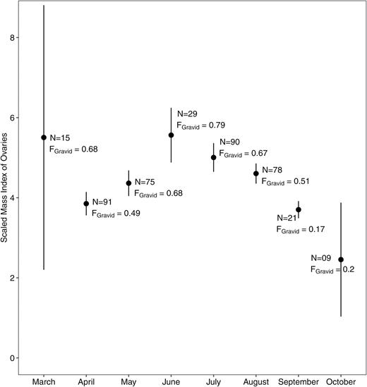
Mean values (± SE) of the SMIorgan of females Xenopus laevis captured in 2014. The number of individuals (N) and the proportion of gravid females (FGravid) captured each month is mentioned close to the dot of each month.
Spatial variation in resource allocation
In 2015, the proportion of gravid females was 66.26% for the core, 78.43% for the intermediate and 51.67% for the edge cluster. According to the linear mixed models, allocation to reproduction for females decreased from the range core to the intermediate [SMIorgan (Core) − SMIorgan (Inter) = 1.46] and edge [SMIorgan (Core) – SMIorgan (Edge) = 0.92] ranges (Fig. 3 and Table 1). In males, SMIorgan was not significantly higher (Table 1) in the core cluster than in the intermediate cluster [SMIorgan (Core) − SMIorgan (Inter) = 0.34] and significantly higher (Table 1) at the core than at the range edge [SMIorgan (Core) – SMIorgan (Edge) = 0.37]. The decrease in SMIorgan mainly concerned the gonad relative mass for females, whereas, for males, both testicles and adipose tissue masses were reduced at the range edge (Table 2).
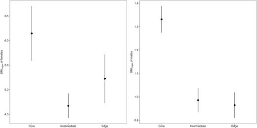
Reproductive investment of Xenopus laevis in the core, intermediate and edge clusters as represented by the SMIorgan (mean ± SE) of females (left) and males (right).
Results of the linear mixed models performed to test the spatial variation in reproductive allocation across the colonized range of Xenopus laevis in France
| Model formula: SMIorg ~ cluster + month + SMIbody+ ~1 |cluster/pond | ||||||
|---|---|---|---|---|---|---|
| Effects | Estimate | SE | df | t-value | P-value | |
| Females | Intercept | 0.853 | 0.849 | 245 | 1.004 | 0.316 |
| Cluster core vs. edge | −2.359 | 0.923 | 23 | −2.555 | 0.018 | |
| Cluster core vs. inter | −2.427 | 0.989 | 23 | −2.454 | 0.022 | |
| Month | −0.286 | 0.769 | 245 | −0.272 | 0.710 | |
| SMIbody | 0.106 | 0.009 | 24 | 11.989 | < 0.001 | |
| Random | ||||||
| Cluster/pond | 1.235 | 2.844 | – | – | – | |
| Males | Intercept | 0.142 | 0.010 | 377 | 1.364 | 0.173 |
| Cluster core vs. edge | −0.025 | 0.010 | 24 | −2.384 | 0.025 | |
| Cluster core vs. inter | −0.008 | 0.012 | 24 | −0.701 | 0.490 | |
| Month | −0.003 | 0.006 | 377 | −0.447 | 0.655 | |
| SMIbody | 0.003 | < 0.001 | 377 | 14.380 | < 0.001 | |
| Random | ||||||
| Cluster/pond | 0.017 | 0.035 | – | – | – | |
We tested a model for each sex, to estimate the variation of SMIorgan according to the cluster, with the month of capture and the SMIbody as covariates. The pond nested in the cluster was used as a random effect.
Mean values and SE obtained for each sex for the SMI of gonads, adipose tissue and entire reproductive organ in the three clusters
| Core | Intermediate | Edge | |
|---|---|---|---|
| Females | |||
| SMIgonad | 5.36 ± 0.56 | 3.80 ± 0.29 | 4.09 ± 0.46 |
| SMIadipose | 1.02 ± 0.12 | 0.88 ± 0.10 | 1.71 ± 0.15 |
| SMIorgan | 6.14 ± 0.56 | 4.67 ± 0.25 | 5.22 ± 0.49 |
| Males | |||
| SMIgonad | 0.11 ± 0.004 | 0.11 ± 0.004 | 0.08 ± 0.003 |
| SMIadipose | 1.22 ± 0.06 | 0.88 ± 0.05 | 0.89 ± 0.05 |
| SMIorgan | 1.33 ± 0.06 | 0.99 ± 0.05 | 0.96 ± 0.06 |
DISCUSSION
In this study, we observed a modification of the reproductive investment of X. laevis in Western France. This modification consists in a decrease of the relative mass of reproductive organs during the first part of the peak of reproduction from the core of the colonized range to its periphery.
Determination of the breeding season
According to our results based on the data collected in 2014, the proportion of sexually active females varied between March and October in the French population. Reproductive activity peaked for 3 months between April and June. In South Africa, the breeding period lasts 3–5 months (Deuchar, 1975). The maximal breeding activity lasts only 2–3 months in California, but reproduction can occur from January to November (McCoid & Fritts, 1989). The duration of the optimal breeding period in France and South Africa cannot be strictly compared because Deuchar (1975) only mentioned the breeding period and did not define the optimal breeding period in itself. In California, water temperature in ponds reaches 20 °C each month of the year. Such a high-temperature regime could favour year-round reproduction (McCoid & Fritts, 1989). In France, a drop in temperature could explain the sharp decrease in the proportion of gravid females and the relative gonad mass at the beginning of autumn when air temperature usually remains below 20 °C. Temperature, among others, affects the variation of food abundance, which could be a crucial factor for the sexual activity of the species (Holland & Dumont, 1975; Girish & Saidapur, 2000). In 2015, to study reproductive allocation, we only considered April and May. We excluded June because most females captured at this moment are likely to have already laid some eggs during the previous months.
Spatial variation in resource allocation
In 2015, we found that at the beginning of the optimal breeding period, the proportion of gravid females was lower at the range edge, but the effect was rather weak. A lower frequency of reproductive females has already been observed in an invasive amphibian during range expansion (Hudson et al., 2015). However, these authors were not able to unambiguously link this pattern to a lower investment in reproduction at the range edge because their data were not initially collected for that purpose. Also, in our study, we cannot provide an unambiguous conclusion as the non-gravid females that we caught may have bred earlier in spring or may reproduce later in the summer. Females from the core area may also be able to restart ovary development earlier than females from the range edge but laboratory studies remain necessary to test this hypothesis.
The masses obtained with the SMI appeared much more informative, with significantly lower values at the range edge compared to the core area for both sexes. These modifications concerned the testicles and adipose tissues for males, both reduced at the range edge. In anurans, this tissue is crucial to allow spermatogenesis in males and the priming of sexual behaviour (Iela et al., 1979; Grafe, Schmuck & Linsenmair, 1992). At the opposite, no changes in adipose tissue mass have been detected for females. Its extent is minimal during the breeding season (Iela et al., 1979), and there is a negative correlation between adipose tissue and ovary mass (Girish & Saidapur, 2000). The lack of differences in adipose tissue mass for females between the range edge and the core area could be explained by the time of the study, that is the first 2 months of the peak of reproductive activity. For both sexes, stronger differences are expected when the development of the adipose tissue is maximal.
The results of our study are corroborated by the increased allocation to dispersal observed in the same invasive population of X. laevis (Louppe et al., 2017). A study using individual-based models suggested that resource allocation may change depending on the presence, the reproductive rate and the competitive ability of native competitors (Burton et al., 2010). At low density of competitors at the range margin, resource allocation to competitive ability is minimal, while resources allocated to dispersal and reproduction are maximal. At higher density of competitors at the range core, allocation to reproduction decreases when competitors exhibit high reproductive rate and competitive ability. This trait has been studied most commonly in invasive plants (Strauss et al., 2002) and is defined as the effect of an individual on resources and its response to resource deficiency (Goldberg, 1990). It influences the survival probability of individuals as a lower investment in competitive ability leads to a reduced survival in high-density conditions (Burton et al., 2010).
In the colonized area, the aquatic habitats used by X. laevis are occupied by several native amphibian species that breed during the same period of the year (Lescure & de Massary, 2012). During field work, we observed native amphibians such as Pelophylax sp. in high densities in every pond. Other species (e.g. Rana dalmatina, Lissotriton helveticus, Triturus cristatus) were often observed at lower densities. Unfortunately, even if impacts of X. laevis on other amphibians have already been shown (Lillo, Faraone & Lo Valvo, 2011), no study has assessed the competition between invasive and native amphibians. Competition through trophic resource access is likely to occur (JC et al., pers. observ.). Further investigations testing the impact on native amphibians may provide some clarification about this issue.
Because females lay eggs in groups of one, two or three eggs (Crump, 2015), it is not possible to tell whether a female has already laid some eggs. We limited this effect by analysing data collected during the first 2 months of the peak of reproductive activity. It is also important to notice that every female is subject to this effect irrespective of the locality where they are captured. Consequently, this effect should not drastically alter the conclusions of this study, but it should be taken into account in future studies using the results from the present study (i.e. care should be taken in interpreting these data as absolute values of reproductive investment). The pattern of variation in reproductive organ mass that we observed is primarily expected to reflect changes in the allocation of resources to different life-history traits. However, the phenomenon called gene surfing, that is the fact that mutations occurring on the range edge travel with the wave front and induce mutant populations (Edmonds, Lillie & Cavalli-Sforza, 2004), could provide an alternative explanation. This process may sort a different pool of alleles in different directions as propagules are loosely connected at the margins of an expanding range (Excoffier et al., 2009). Genetic analyses may help to solve this issue. Sampling transects pointing away from the range core in different directions would certainly also help to provide more robust conclusions. Finally, common garden studies on resource allocation in expanding populations have already demonstrated that heritability could have an effect on the observed pattern for a life-history trait (Brown, Phillips & Shine, 2014). The African clawed frog is an interesting model to address this issue because the ecological conditions (climate, communities) encountered in its native range and the colonized areas differ. This species, by offering intra-specific comparisons across populations introduced independently in different countries, may bring insights into the processes of range expansion and invasion.
ACKNOWLEDGEMENTS
We gratefully thank the two anonymous reviewers of this study and Prof. John A. Allen who led the reviews of our study. We thank the Agglomération du Bocage Bressuirais and the Communauté de Communes du Thouarsais for their help during the fieldworks. We also thank the Société Herpétologique de France for providing us the occurrence data of Xenopus laevis. This research was funded by the ERA-Net BiodivERsA, with the national funders ANR, DFG, BELSPO and FCT, as part of the 2013 BiodivERsA call for research proposals. INVAXEN ‘Invasive biology of Xenopus laevis in Europe: ecology, impact and predictive models’ project ANR-13-EBID-0008-01. AH, JS and JC conceived the study. JC and VB collected data in the field. JC, VB and JS analysed data, and all authors contributed to the writing of the paper.
References
