


Abstract
We have studied the effects of various initial mass functions (IMFs) on the chemical evolution of the Sagittarius dwarf galaxy (Sgr). In particular, we tested the effects of the integrated galactic initial mass function (IGIMF) on various predicted abundance patterns. The IGIMF depends on the star formation rate and metallicity and predicts less massive stars in a regime of low star formation, as it is the case in dwarf spheroidals. We adopted a detailed chemical evolution model following the evolution of α-elements, Fe and Eu, and assuming the currently best set of stellar yields. We also explored different yield prescriptions for the Eu, including production from neutron star mergers. Although the uncertainties still present in the stellar yields and data prevent us from drawing firm conclusions, our results suggest that the IGIMF applied to Sgr predicts lower [α/Fe] ratios than classical IMFs and lower [hydrostatic/explosive] α-element ratios, in qualitative agreement with observations. In our model, the observed high [Eu/O] ratios in Sgr is due to reduced O production, resulting from the IGIMF mass cut-off of the massive oxygen-producing stars, as well as to the Eu yield produced in neutron star mergers, a more promising site than core-collapse supernovae, although many uncertainties are still present in the Eu nucleosynthesis. We find that a model, similar to our previous calculations, based on the late addition of iron from the Type Ia supernova time-delay (necessary to reproduce the shape of [X/Fe] versus [Fe/H] relations) but also including the reduction of massive stars due to the IGIMF, better reproduces the observed abundance ratios in Sgr than models without the IGIMF.
1 INTRODUCTION
The Sagittarius (Sgr) dwarf galaxy was the last classical dwarf spheroidal (dSph) discovered before the advent of the Sloan Digital Sky Survey. Its discovery was made by Ibata, Gilmore & Irwin (1994) and it was identified while performing a spectroscopic radial velocity survey of the Galactic bulge stars (Ibata et al. 1997). Its heliocentric distance (D⊙ = 26 ± 2 kpc; from Simon et al. 2011) makes it the second closest known satellite galaxy of the Milky Way (MW) and, because of the strong tidal interaction suffered by the Sgr dSph during its orbit, it has left behind a well-known stellar stream (Ibata et al. 2001; Majewski et al. 2003; Belokurov et al. 2006), whose chemical characteristics have been recently studied and compared with the ones of the Sgr main body and other dSph galaxies by de Boer et al. (2014). The Sgr dwarf galaxy has been classified as a dSph because of its very low central surface brightness (μV = 25.2 ± 0.3 mag arcsec−2; from Majewski et al. 2003), its very small total amount of gas (|$M_{{\rm H\,\small {i},obs}}\sim 10^4\,\mathrm{M}_{\odot }$|; from McConnachie 2012) and because of the age and metallicity of its main stellar population, which dates back to the age of the Universe and it is on average very iron poor. Chemical abundances in Sgr have been measured by many authors up to now (see Lanfranchi, Matteucci & Cescutti 2006, and references therein). Most of these studies have shown that the abundance patterns in Sgr are different than those in the MW.
This work aims at testing the suggestions of McWilliam, Wallerstein & Mottini (2013), which claimed that the α-element deficiencies observed in the Sgr dSph galaxy cannot be explained only by means of the time-delay model (Tinsley 1979; Greggio & Renzini 1983; Matteucci & Greggio 1986) but they rather result from an initial mass function (IMF) deficient in the highest mass stars. On the other hand, Lanfranchi & Matteucci (2003, 2004) suggested that the low values of the [α/Fe] ratios,1 as observed in dSphs, can be interpreted as due to the time-delay model (α-elements produced on short time-scales by core-collapse SNe and Fe by SNe Ia with a time delay) coupled with a low star formation rate (SFR), assuming a Salpeter (1955) IMF.
McWilliam et al. (2013) also suggested that the Eu abundances in the Sgr galaxy might be explained by core-collapse SNe, whose progenitors are stars less massive than the main oxygen producers, as previously envisaged also by Wanajo et al. (2003). Since many studies of nucleosynthesis have pointed out the difficulty of producing r-process elements during SN explosions (Arcones, Janka & Scheck 2007), in this work, we test different scenarios for the Eu production, both the one in which Eu is produced by core-collapse SNe and the most recent one, where the Eu is synthesized in neutron star mergers (NSMs; Korobkin et al. 2012; Tsujimoto & Shigeyama 2014; Shen et al. 2014; van de Voort et al. 2015). The latter scenario was recently explored in the context of a detailed chemical evolution model by Matteucci et al. (2014), where they were able to well match the [Eu/Fe] abundance ratios observed in the MW stars.
Here, we study the detailed chemical evolution of Sgr by comparing the effect of the integrated galactic initial mass function (IGIMF, in the formulation of Recchi et al. 2014, hereafter R14) with the predictions of the canonical Salpeter (1955) and Chabrier (2003) IMFs. The main effect of the metallicity-dependent IGIMF of R14 is a dependence of the maximum possible stellar mass, that can be formed within a stellar cluster, on the [Fe/H] abundance and on the SFR, especially if the latter is very low. Since the dSphs turn out to have been characterized by very low SFRs, the effect of the IGIMF on their evolution is expected to be important. In this way, we will be able to test if the hypothesis of McWilliam et al. (2013) is correct.
In the past, the effect of the IGIMF in the chemical evolution of elliptical galaxies has been studied by Recchi, Calura & Kroupa (2009), while Calura et al. (2010) modelled the chemical evolution of the solar neighbourhood when assuming the IGIMF. The originality of this work resides also in the fact that we test the effect of a metallicity-dependent IMF, a study never done before in the framework of a detailed chemical evolution model. As a further element of originality, we include for the first time the Eu from NSMs in a chemical evolution model of a dSph galaxy.
Our work is organized as follows. In Section 2, we describe the metallicity-dependent IGIMF formalism that we include in our models. In Section 3, the data sample is presented. In Section 4, we describe the chemical evolution model adopted for the Sgr dSph and in Section 5 we show and discuss the results of our study. Finally, in Section 6, we summarize the main conclusions of our work.
2 THE INTEGRATED GALACTIC INITIAL MASS FUNCTION
- The mass spectrum of the embedded stellar clusters is assumed to be a power law, |$\xi _{{\rm ecl}}\propto M_{{\rm ecl}}^{-\beta }$|, with a slope β = 2 (Zhang & Fall 1999; Recchi et al. 2009). In accordance with the mass of the smallest star-forming stellar cluster known (the Tauris–Auriga aggregate), we assumed Mecl, min = 5 M⊙, whereas the upper mass limit of the embedded cluster is a function of the SFR (Weidner & Kroupa 2004):with A = 4.83 and B = 0.75.(2)\begin{equation} \log {M_{{\rm ecl,max}}} = A + B\,\log {\frac{\psi (t)}{\mathrm{M}_{\odot }{\rm yr}^{-1}}}, \end{equation}
- Within each embedded stellar cluster of a given mass Mecl and [Fe/H] abundance, the IMF is assumed to be invariant. In our study, we assume an IMF which is defined as a two-slope power law:where α1 = 1.30 and α2 = 2.35 as in the original work of Weidner & Kroupa (2005), and α2 = 2.3 + 0.0572· [Fe/H] in the mild formulation of R14. The latter relation was adapted by R14 from the original work of Marks et al. (2012). It turns out from equation (3) that the overall [Fe/H] dependence entirely resides in the slope of the IMF of the high-mass range. The maximum stellar mass mmax that can occur in the cluster and up to which the IMF is sampled, is calculated according to the mass of the embedded cluster, Mecl; furthermore, mmax must be in any case smaller than the empirical limit, which here has been assumed to be 150 M⊙ (see for more details, Weidner & Kroupa 2004). The mmax–Mecl relation is simply due to the fact that, in the case of very low SFRs, the small clusters may not have enough mass to give rise to very massive stars; on the other hand, in the case of large SFRs, the maximum possible mass of the embedded clusters may be very large and so very massive stars are able to originate (see R14). So mmax depends both on the SFR and, to a lesser extent, on the [Fe/H] abundance of the parent galaxy.(3)\begin{equation} \phi (m)= \left\lbrace \begin{array}{l l}A\,m^{-\alpha _{1}} & \quad {\rm for}\ 0.08 \mathrm{M}_{\odot } \le m < 0.5 \mathrm{M}_{\odot }\\ B\,m^{-\alpha _{2}} & \quad {\rm for}\ 0.5 \mathrm{M}_{\odot } \le m < m_{{\rm max}}, \end{array} \right. \end{equation}
It is worth remarking that recent studies (Weidner, Kroupa & Pflamm-Altenburg 2011; Kroupa et al. 2013; Weidner et al. 2013) suggest that the star cluster IMFs can become top-heavy at SFRs larger than ∼10 M⊙ yr−1. This range of SFRs is clearly out of reach for Sgr, therefore we have neglected this modification of the IGIMF theory in our study.
In Fig. 1, we show what is the effect of the dependence of the IGIMF upon the SFR. For very low SFRs (≤1 M⊙ yr−1), the IGIMF turns out to be very much truncated and the maximum mass that can be formed strongly depends on the SFR. This is due to the fact that, in galaxies with a low SFR, the mass distribution function of the embedded clusters is truncated at low values of Mecl (see equation 2) and small embedded clusters cannot produce very massive stars.
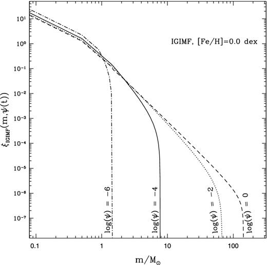
In this figure, we show the predicted IGIMF, ξIGIMF, as a function of the stellar mass m in the case of solar iron abundance and for various SFRs: from ψ(t) = 10−6 M⊙ yr−1 up to ψ(t) = 1 M⊙ yr−1. The net effect of lowering the SFR is to truncate the IGIMF towards lower stellar masses.
In Fig. 2, we illustrate how mmax is determined both by the SFR and by the [Fe/H] abundance. The effect of the [Fe/H] dependence is clearly opposite to that of the SFR dependence. As time passes by, one would expect that the iron content within the galaxy insterstellar medium (ISM) increases; so, in this formulation, if the SFR is constant, the maximum stellar mass that can be formed within each embedded cluster is expected to decrease in time. In any case, it is worth noting that the dependence of mmax upon the SFR is much stronger than the dependence upon [Fe/H] when the SFRs under play are extremely low.
![This figure shows how the maximum stellar mass (on the y-axis) varies as a function of the SFR (on the x-axis) and as a function of the [Fe/H] abundance (colour-coding: from −7 dex up to 1 dex). Increasing the [Fe/H] abundance has an opposite effect on mmax with respect to the increasing of the SFR.](https://oup.silverchair-cdn.com/oup/backfile/Content_public/Journal/mnras/449/2/10.1093_mnras_stv357/2/m_stv357fig2.jpeg?Expires=1716437480&Signature=J5P7OwMNoVciGEemtjP391Hqc5EJgnXQ4Rm56Orwk5DDk070jtVndAk6SRtmh~94x7a7AmAoakds1v3deKML5zSpJ46~u4kg3EaW8HhJvdiYafMzqWe1QcsyiY82dv63Hoy-18wvZhyzPTfTnutbHUU7srV6fwwYSd7xGNhMLyPO8KkfTtQrgNqKIRhT7~j~8DNYVwnYOwC5TxSbWg6~NAVvDndro0V7FmwwF9VyAJUEHot5hGsMABCVnKMvHsmrkInG7gsnl1JbuU-9NFb32Mj-jklAilPOxmNu0WfClMz6TE3-GO5U5Ua86DXrvBQWkVmCRdmWKTL4Jr7XehNhBw__&Key-Pair-Id=APKAIE5G5CRDK6RD3PGA)
This figure shows how the maximum stellar mass (on the y-axis) varies as a function of the SFR (on the x-axis) and as a function of the [Fe/H] abundance (colour-coding: from −7 dex up to 1 dex). Increasing the [Fe/H] abundance has an opposite effect on mmax with respect to the increasing of the SFR.
3 DATA SAMPLE
We use the data set of chemical abundances from the works of Bonifacio et al. (2000, 2004), Sbordone et al. (2007) and McWilliam et al. (2013). Bonifacio et al. (2000) derived the abundances of many chemical elements for two giant stars in Sgr, observed with the high-resolution Ultraviolet and Visual Echelle Spectrograph (UVES) at the Kueyen-Very Large Telescope (VLT). Bonifacio et al. (2004) did a similar work as Bonifacio et al. (2000), including the two stars previously analysed. From the former work, we took the abundances of Eu, while from the latter one we took the abundances of Mg and O. Sbordone et al. (2007) presented the chemical abundances of 12 red giant stars belonging to the Sgr main body and the chemical abundances of five red giant stars belonging to the Sgr globular cluster Terzan 7, acquired with the UVES at the European Southern Observatory (ESO) VLT. McWilliam et al. (2013) derived the abundances of several chemical elements from high-resolution spectra of three stars lying on the faint red giant branch of M54, which is considered the most populous globular cluster of Sgr, lying in the densest regions of the galaxy. McWilliam et al. (2013) acquired the spectra using the Magellan Echelle spectrograph (MIKE) and their three stars were confirmed from their kinematics to belong to the Sgr galaxy by Bellazzini et al. (2008). McWilliam et al. (2013) found their chemical abundances of Eu and Mg consistent with those of Bonifacio et al. (2000, 2004).
4 THE CHEMICAL EVOLUTION MODEL
4.1 The general model for dSphs
In this work, we use a similar numerical code as described in Lanfranchi & Matteucci (2004) and then adopted also in Lanfranchi et al. (2006). The Sgr dSph is assumed to assemble from infall of primordial gas into a pre-existing dark matter (DM) halo, in a relatively short typical time-scale. The infall gas mass has been set to Minf = 5.0 × 10⁸ M⊙ and the infall time-scale has been set to τinf = 0.5 Gyr, following the results of Lanfranchi et al. (2006). We assume Sgr to have a massive and diffuse DM halo, with a mass MDM = 1.2 × 10⁸ M⊙ (Walker et al. 2009) and S ≡ rL/rDM = 0.1, where rL = 1550 pc (Walker et al. 2009) represents the effective radius of the baryonic matter and rDM is the core radius of the DM halo. We need the latter quantities in order to compute the potential well of the gas and the time of the onset of the galactic wind, which is triggered by the energy released into the ISM by the stellar winds and by the core-collapse (Type II, Type Ib, Type Ic) and Type Ia SNe (see for more details, Bradamante, Matteucci & D'Ercole 1998; Yin, Matteucci & Vladilo 2011). Once the wind has started,2 the intensity of the outflow rate is directly proportional to the SFR.
The galaxy is modelled as a one-zone within which the mixing of the gas is instantaneous and complete and the stellar lifetimes are taken into account. We include the metallicity-dependent stellar yields of Karakas (2010) for the low- and intermediate-mass stars. For massive stars, we assume the He, C, N and O stellar yields at the various metallicities of Meynet & Maeder (2002), Hirschi, Meynet & Maeder (2005), Hirschi (2007) and Ekström et al. (2008) and, for heavier elements, the yields of Kobayashi et al. (2006). Finally, we include the yields of Iwamoto et al. (1999) for the Type Ia SNe. We assume the same stellar yields as Matteucci et al. (2014, see also Romano et al. 2010 for a detailed description). It is worth noting that the yields of Romano et al. (2010) have been selected because they are, at the present time, the best in order to reproduce the abundance patterns in the solar vicinity.
We test in our model, separately, three different Eu nucleosynthetic yields:
the yields of Cescutti et al. (2006, model 1, table 2), in which the Eu is produced by core-collapse SNe, whose progenitors are massive stars with mass in the range M = 12–30 M⊙;
the yields of Ishimaru et al. (2004), which can be found tabled in Cescutti et al. (2006, model 4, table 2), where the Eu is produced by massive stars with mass in the range M = 8–10 M⊙, exploding as core-collapse SNe;
the yield prescriptions of Matteucci et al. (2014), where we address the reader for details, for the Eu produced by NSMs.3 The first case we test is the model Mod3NS′ (see fig. 6 of Matteucci et al. 2014), where we assume that the Eu mass per NSM event is MEu,NSM = 3.0 × 10⁻⁶ M⊙; the progenitors of neutron stars lie in the range 9–50 M⊙; the fraction of binary systems in this mass range becoming NSMs is αNSM = 0.02, and the time delay for NS coalescence is ΔtNSM = 1 Myr (we check also 100 Myr as shown in Section 5.1). Moreover, we test also a model with MEu,NSM = 10−5 M⊙ per merger event, and the other parameters being the same as Mod3NS′. This value of the Eu yield is in agreement with the results of recent calculations (Bauswein et al. 2014; Just et al. 2015; Wanajo et al. 2014).
4.2 The model for Sagittarius
In this study, we follow the results of Lanfranchi et al. (2006), which provide an estimate of the parameters of the chemical evolution model for Sgr able to reproduce the observational data. They found that Sgr should have been characterized by intermediate values of the star formation efficiencies ν, included between 1 and 5 Gyr−1, and by intense galactic winds, with efficiencies λ varying between 9 and 13 Gyr−1. Lanfranchi et al. (2006) assumed a constant Salpeter (1955) IMF.
In accordance to the observations, we assume that Sgr is composed of two distinct stellar populations, one of old age ≥10 Gyr (the blue horizontal branch population discovered by Monaco et al. 2003) and one of intermediate age, which date back to 8.0 ± 1.5 Gyr (the so-called Population A, studied by Bellazzini et al. 2006). So we adopt for the galaxy a star formation history with two separate episodes, the first one occurring between 0 and 4 Gyr since the beginning of the galaxy evolution, the second one between 4.5 and 7.5 Gyr. Thus, according to these observational evidences, the star formation is set to zero outside those time intervals. During the star formation episodes, the SFR follows the Schmidt law (see equation 5).
5 RESULTS
This work is based on the chemical evolution model described in Section 4 and our aim is to investigate the effect of three different IMFs: the canonical Salpeter (1955), the Chabrier (2003) IMF and the metallicity-dependent IGIMF of R14.
The galaxy is always predicted to possess at the present time a very small total amount of gas. In particular, the total H i mass results |$M_{{\rm H\,\small {i}}}\approx 1.8\times 10^{4}\,\mathrm{M}_{\odot }$| with the Chabrier (2003) IMF, |$M_{{\rm H\,\small {i}}}\approx 1.3\times 10^{4}\,\mathrm{M}_{\odot }$| with the Salpeter (1955) IMF and |$M_{{\rm H\,\small {i}}}\approx 1.8\times 10^{4}\,\mathrm{M}_{\odot }$| with the IGIMF. All the latter quantities are almost in agreement with the upper limit of the total H i mass derived by Koribalski, Johnston & Otrupcek (1994), which is |$M_{{\rm H\,\small {i},obs}}\sim 10^{4}\,\mathrm{M}_{\odot }$|.
The model with the IGIMF predicts the largest final total stellar mass for the galaxy, which is M⋆, fin ≈ 1.1 × 10⁸ M⊙. In fact, the model with the Salpeter (1955) and Chabrier (2003) IMFs predict M⋆, fin ≈ 7.9 × 10⁷ M⊙ and M⋆, fin ≈ 5.2 × 10⁷ M⊙, respectively, which have the same order of magnitude of the observed total stellar mass M⋆ ∼ 2.1 × 10⁷ M⊙ (see McConnachie 2012 and references therein). In this study, we have neglected the fact that Sgr has lost many stars after its SF ceased; this may explain why the actual stellar mass predicted by our chemical evolution models is larger than the present-day observed mass.
The model with the IGIMF predicts the galactic wind to develop for the first time at tGW = 30 Myr while the model with the Salpeter (1955) and the Chabrier (2003) IMFs predict the onset of the galactic wind at tGW = 25 and 20 Myr, respectively. Since we assume the SFR to proceed since the beginning, the retarded onset of the galactic wind with the IGIMF is likely due to the strong truncation of IGIMF itself, which inhibits the formation of very massive stars, the ones having the shortest typical lifetimes and exploding as core-collapse supernovae. This can be confirmed by the intensity of the SFRs under play; if they are ≤1 M⊙ yr−1, then the truncation is important. By looking at Fig. 3, where the predicted trend of the SFR is plotted as a function of time, it turns out that the predicted SFRs in Sgr are always much lower than 1 M⊙ yr−1. The temporal evolution of the maximum stellar mass that can be formed during the star formation activity, in the case of the IGIMF, is shown in Fig. 4. The steep increasing trend of mmax at the beginning is due to the rapid increase of the SFR during the initial infall event. Then, mmax decreases because of the declining SFR. The [Fe/H] dependence is crucial during the initial infall event, when the [Fe/H] abundance rapidly increases, counterbalancing the SFR dependence and preventing the IGIMF to reach masses very close to the empirical limit of 150 M⊙. In fact, the bulk of chemical enrichment in this galaxy occurs in the first Gyr of its evolution; then, the age–metallicity relation becomes much more shallow and the main role is played by the SFR, which decreases very steeply. In Fig. 5, we report the age–metallicity relations predicted by assuming the different IMFs. The small fluctuations visible in Fig. 5 are due to the bursting mode of star formation and the alternance of SF and quiescent periods.
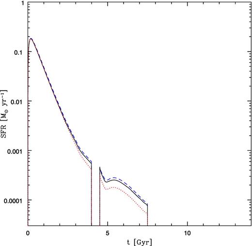
In this figure, we compare the temporal evolution of the SFR as predicted by assuming the metallicity-dependent IGIMF of R14 (black solid line) with the same quantity predicted by assuming the Salpeter (1955, dotted line in red) and Chabrier (2003, blue dashed line) IMFs. The trend of the SFR traces that of the gas mass content within the galaxy. In all the cases considered here, the SFR is always much lower than 1 M⊙ yr−1. Notice that the various curves almost overlap. This is due to the fact that the IMF has little effect on the global mass budget.
![Given the temporal evolution of the SFR and of the [Fe/H] abundance predicted by our chemical evolution model, this figure reports how the maximum stellar mass that can be formed at every time t evolves as a function of the time itself, when assuming the metallicity-dependent IGIMF of R14. It is clear how much the truncation becomes important when the IGIMF is adopted in a detailed chemical evolution model of a galaxy with very low SFRs.](https://oup.silverchair-cdn.com/oup/backfile/Content_public/Journal/mnras/449/2/10.1093_mnras_stv357/2/m_stv357fig4.jpeg?Expires=1716437480&Signature=u4VMYTbJBSltNRaAM6iyjIs5R7iogWtnwvqLChUgUf8NKPqgjoy7EAtIwgN1FNArFqq7DYwE-zUXEqrhugN29e12ETNU2lWfEfy-BLyTMIJ~6jhSmRVmy87CntO-evd8xA-fxFQ-Q4a0titlktOaXg-UTMzjjdQ9hjhdgpQjb9Pu7il5MYWAy9KiHw8NtXYBy~0siBQ56VQCg-Llhg2nGJ0E5khMnYwKPIjA8ETqPiJK8aCcQMVYmBpoLN0zcCIYAu0SOi7VM3C5HDu54TIqCA8ytw6btqiuGTXz8aSq~KvQcp901tw58oOlRM5P0M0jbW5DFN9TMP6tyB-4zLO9eQ__&Key-Pair-Id=APKAIE5G5CRDK6RD3PGA)
Given the temporal evolution of the SFR and of the [Fe/H] abundance predicted by our chemical evolution model, this figure reports how the maximum stellar mass that can be formed at every time t evolves as a function of the time itself, when assuming the metallicity-dependent IGIMF of R14. It is clear how much the truncation becomes important when the IGIMF is adopted in a detailed chemical evolution model of a galaxy with very low SFRs.
![In this figure, the predicted age–metallicity relation is shown. The y-axis reports the [Fe/H] abundance of the galaxy ISM as predicted by our chemical evolution models, while the x-axis reports the time in Gyr since the beginning of the galaxy evolution. The iron content within the ISM increases very steeply in the first billion years, then its trend flattens. The different IMFs considered in this work predict very similar age–metallicity relations. We remark on the fact that the [Fe/H] abundance in this figure refers to the abundance in the ISM; if one wants to see how many stars formed at a given time and therefore at a given [Fe/H] of the ISM, one should look at the stellar MDF (see Section 5). The lines correspond to the same IMFs as in Fig. 3.](https://oup.silverchair-cdn.com/oup/backfile/Content_public/Journal/mnras/449/2/10.1093_mnras_stv357/2/m_stv357fig5.jpeg?Expires=1716437480&Signature=aUFxr-oiaYIddHieJ9v61c6cqXIXIfXqd8EzCP4jgwV5btkmwl2ZzX68ZfrM6gEazUKthDBqwYya4Q~1Xey25uM-M7gFyqzudHYaSfacQ0AgYloOizIXz5bwm8sxNBmoYhRqQwXsLaJ-cq9cKSBueQHMHY3FgLmuqx3oz21IAj04PZDHSBYzB9x-Wc11MjDg~t0~YyVZ7rmmblB~iQ6EDkOXkBqLcGfwVhKqDXKx-MRav0kJQorLF~mIsib1kY1DnD6VBxaG3PMcA7qe4jgsIfJLOPQGbo6R5aCn8q1BKvfToX3L9fYNxFj9vAr2boDuqbW2AcmWuO~S6P44Cf8cIQ__&Key-Pair-Id=APKAIE5G5CRDK6RD3PGA)
In this figure, the predicted age–metallicity relation is shown. The y-axis reports the [Fe/H] abundance of the galaxy ISM as predicted by our chemical evolution models, while the x-axis reports the time in Gyr since the beginning of the galaxy evolution. The iron content within the ISM increases very steeply in the first billion years, then its trend flattens. The different IMFs considered in this work predict very similar age–metallicity relations. We remark on the fact that the [Fe/H] abundance in this figure refers to the abundance in the ISM; if one wants to see how many stars formed at a given time and therefore at a given [Fe/H] of the ISM, one should look at the stellar MDF (see Section 5). The lines correspond to the same IMFs as in Fig. 3.
The core-collapse SN rate as a function of time is shown in Fig. 6. The progenitors of core-collapse SNe are assumed to be massive stars with mass M > 8 M⊙, which have very short typical lifetimes since star formation, in the range 1 Myr < τM < 35 Myr. As one can see from the figure, the IGIMF predicts numbers of core-collapse SNe per unit time which are always lower than the ones predicted by the classical IMFs. On the other hand, among the IMFs here considered, the highest number of stars over the entire high-mass range originate when assuming the Chabrier (2003) IMF (see also Romano et al. 2005). In fact, the Chabrier (2003) IMF for M ≥ 1 M⊙ has a slope αChab. = −2.3 (see equation 8), which is flatter than the Salpeter (1955) one (αSal. = −2.35, see equation 7). For this reason, the core-collapse SN rate with the Chabrier (2003) exceeds the other.
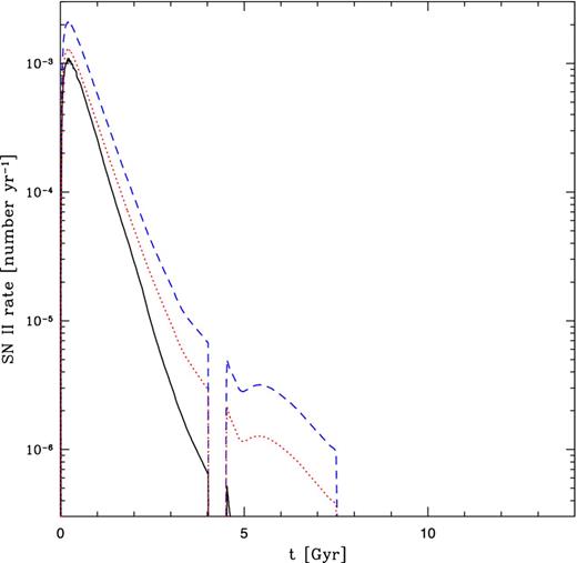
This figure reports the core-collapse SN rate predicted as a function of the time. Because of the truncation of the IGIMF, the core-collapse SN rate predicted by the IGIMF is always lower than the one predicted by the classical IMFs. The lines correspond to the same IMFs as in Fig. 3.
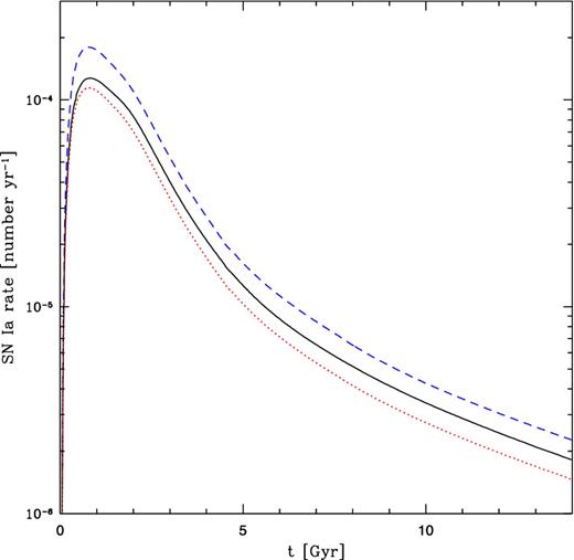
In Fig. 7, we report the predicted Type Ia SN rate as a function of time. We assume Type Ia SNe to originate from white dwarfs in binary systems exploding by C-deflagration. We adopt the so-called single-degenerate model, with the same prescriptions of Matteucci & Recchi (2001). According to this particular progenitor model, a degenerate C–O white dwarf (the primary, initially more massive, star) accretes material from a red giant or main-sequence companion (the secondary, initially less massive, star); in summary, when the white dwarf reaches the Chandrasekhar mass, the C-deflagration occurs and the white dwarf explodes as a Type Ia supernova (for more details, see Matteucci 2001). Depending primarily on the mass of the secondary star, which is the clock for the explosion, Type Ia SNe can explode over a very large interval of time-scales since the star formation, which can vary between 35 Myr and the age of the Universe. By looking at Fig. 7, the Type Ia SN rate with the Chabrier (2003) IMF dominates over the other two; in fact, the Chabrier (2003) IMF predicts also a higher number of low- and intermediate-mass stars with M > 1 M⊙ (Romano et al. 2005).
5.1 MDF and chemical abundances
The stellar metallicity distribution function (MDF) predicted by the model with the IGIMF has the peak at [Fe/H] = −0.48 dex, close to the position of the peak predicted by the model with the Salpeter (1955) IMF, which is at [Fe/H] = −0.51 dex. Conversely, the [Fe/H] peak of the MDF with the Chabrier (2003) IMF occurs at [Fe/H] = −0.26 dex, which is much higher than the other two values. This can be seen in Fig. 8 and it is due to the fact that the integrated number of Type Ia and core-collapse SNe with the Chabrier (2003) IMF is much higher than that predicted when assuming the IGIMF or the Salpeter (1955) IMF (see Figs 6 and 7). So, on average, fixing all the other parameters of the model, a quite enhanced iron pollution from SNe is expected when adopting the Chabrier (2003) IMF. Finally, the IGIMF and the Salpeter (1955) IMF predict a [Fe/H] abundance for the peak of the stellar MDF which is in agreement with the mean value 〈[Fe/H]〉 = −0.5 ± 0.2 dex, measured by Cole (2001) for the Sgr main stellar population.
![In this figure, we compare the stellar MDF as predicted by the various models. The theoretical MDFs have been smoothed with a Gaussian function having σ = 0.2. The IGIMF and the Salpeter (1955) IMF predict the MDF to peak at [Fe/H] = −0.48 dex and [Fe/H] = −0.51 dex, respectively, in agreement with the mean value 〈[Fe/H]〉 = −0.5 ± 0.2 dex, measured by Cole (2001). The Chabrier (2003) predicts the peak to occur at [Fe/H] = −0.26 dex. The lines correspond to the same IMFs as in Fig. 3.](https://oup.silverchair-cdn.com/oup/backfile/Content_public/Journal/mnras/449/2/10.1093_mnras_stv357/2/m_stv357fig8.jpeg?Expires=1716437480&Signature=JyclUpBt2Me4jfDa6Hww7zMX~g2xewT8R9wXPzeQRv4RdNoe-4jlLaoWReI56lEJLfXC~wgDL3kBDAnQUKD0xClTygK6yD0AwC8JpSRHXwLIvHeiATFl~biJi8VBtwcA912QncNFtresWVRHA3~3zAnRHnobBuLbb4RMVqbuVspEb4jfwCp9RnkqvUUbn3zuYj3cw65aqaKCAwhEigk5EJWAkS6~MG892DXuud1PVt7E~88wdpFti8lISISx9pwTnRZPLanM97B8HQdSjRYr7pGoJ3QO6QNUr-920SgVdPsSIfFYSurPOHPkv5fqdBTZIUqB-vC3c8FXcXsVFEQZtQ__&Key-Pair-Id=APKAIE5G5CRDK6RD3PGA)
In this figure, we compare the stellar MDF as predicted by the various models. The theoretical MDFs have been smoothed with a Gaussian function having σ = 0.2. The IGIMF and the Salpeter (1955) IMF predict the MDF to peak at [Fe/H] = −0.48 dex and [Fe/H] = −0.51 dex, respectively, in agreement with the mean value 〈[Fe/H]〉 = −0.5 ± 0.2 dex, measured by Cole (2001). The Chabrier (2003) predicts the peak to occur at [Fe/H] = −0.26 dex. The lines correspond to the same IMFs as in Fig. 3.
In Fig. 9, we compare the predicted [α/Fe] abundance ratios as a function of the [Fe/H] abundances with the observational data of Bonifacio et al. (2000, 2004), Sbordone et al. (2007) and McWilliam et al. (2013). We remind the reader that Type Ia SNe enrich the ISM mainly with iron (almost 2/3 of the total content) and iron-peak elements, whereas the α-elements are mainly produced by core-collapse SNe, which also provide some iron, typically ∼1/3 of the total. However, some α-elements, such as the calcium and the silicon, are also synthesized by Type Ia SNe, although in smaller quantities than those coming from core-collapse SNe. We have also to remark the fact that the fraction of the total iron content coming from Type II and Type Ia SNe depends on the assumed IMF and the aforementioned proportions have been calculated by assuming Salpeter-like IMFs (see for more details, Matteucci 2014).
![In this figure, we report the [α/Fe] versus [Fe/H] abundance ratio patterns as predicted by the IGIMF of R14 (black solid line) and by the Salpeter (1955, dashed line in red) and Chabrier (2003, blue dashed line) IMFs. The data are from Bonifacio et al. (2000, 2004, blue squares), Sbordone et al. (2007, grey triangles) and McWilliam et al. (2013, magenta stars). The trend can be easily explained by means of the time-delay model (Matteucci & Brocato 1990; Matteucci & Recchi 2001; Lanfranchi & Matteucci 2004) and by looking at the core-collapse and Type Ia SN rates in Figs 6 and 7, respectively. The lines correspond to the same IMFs as in Fig. 3.](https://oup.silverchair-cdn.com/oup/backfile/Content_public/Journal/mnras/449/2/10.1093_mnras_stv357/2/m_stv357fig9.jpeg?Expires=1716437480&Signature=0jVmKwjawHvNzNw0l2jLqEyo-aNczaWliy78biovopi2WD-UvrD7eR2pqPoCH04xFTiYjWMVmlujhDGzv2ybfwQI25XDXrrarcUQoWLo77fVCDjTLRnmWtDCuea8vRszUbbHpk8jq6YG8qq53zEiNuj4NIryuubCye24uX-IKKAwN4QOE3eyWDfwDIKtRy5cJs9plyfB~60gWGKiZfMiYHUq0RruFpDCh79SHUzhNl1vhmjHqYWbWUeKUb8pMCli95jqAqSomvVL25Lr8NvTqs7l0o81dCfz6urb7mBtkV3pGRDPdH6WUDuMnnabL83We8IMp2Vs-4gjwuK4Rnc9lg__&Key-Pair-Id=APKAIE5G5CRDK6RD3PGA)
In this figure, we report the [α/Fe] versus [Fe/H] abundance ratio patterns as predicted by the IGIMF of R14 (black solid line) and by the Salpeter (1955, dashed line in red) and Chabrier (2003, blue dashed line) IMFs. The data are from Bonifacio et al. (2000, 2004, blue squares), Sbordone et al. (2007, grey triangles) and McWilliam et al. (2013, magenta stars). The trend can be easily explained by means of the time-delay model (Matteucci & Brocato 1990; Matteucci & Recchi 2001; Lanfranchi & Matteucci 2004) and by looking at the core-collapse and Type Ia SN rates in Figs 6 and 7, respectively. The lines correspond to the same IMFs as in Fig. 3.
By looking at Fig. 9, the overall trend predicted by assuming the three different IMFs is quite similar and it can be easily explained by the so-called time-delay model (Matteucci & Brocato 1990; Matteucci & Recchi 2001; Lanfranchi & Matteucci 2004): the decrease of [α/Fe] at very low [Fe/H] is due to the very low SFR under play, which causes Type Ia SNe to be important in the iron pollution when the ISM was not yet heavily enriched with iron by core-collapse SNe; then, the further steepening of [α/Fe] is due to the strong outflow rate. The fundamental role played by the so-called time-delay model in shaping the trend of the [α/Fe] ratios, as a function of [Fe/H], is shown in Fig. 10, where we study the effect of suppressing Type Ia SNe in the chemical enrichment process. As one can see from the figure, if there are no Type Ia SNe, which are the most important Fe producers in galaxies, a truncated IMF such as the IGIMF would never be able to reproduce the data by itself. Furthermore, only by means of Type Ia SNe the galaxy can reach the observed [Fe/H] abundances. In fact, the predicted trend reflects only the contribution of core-collapse SNe to Fe. It is only the contribution of Type Ia SNe that can explain the decrease of [α/Fe] ratios and produce the right amount of Fe.
![In this figure, we study the effect on the predicted [α/Fe] versus [Fe/H] abundance pattern of suppressing Type Ia SNe. The dotted lines correspond to the model with the inclusion of Type Ia SNe, while the solid lines represent the model when the contribution of Type Ia SNe has been suppressed. The dotted lines correspond to the same IMFs as in Fig. 9.](https://oup.silverchair-cdn.com/oup/backfile/Content_public/Journal/mnras/449/2/10.1093_mnras_stv357/2/m_stv357fig10.jpeg?Expires=1716437480&Signature=ssflid~jyHjylEcWMW0f2A6q9YMm6CL1H7xEF5RQLrAqr2Dx7rs8d39Z87OOlNKUbt1m4~c2Nelv2oEJH~Nb-4WIJEQcpBak-2J4YUbSU65x-PrhqmZHF7wi1mJhOo76IIFuIpuHjERyAgwkwQvmiojQF1wXKR30AZpBpf-S9zWiYrXZFSAUScAWi4wgzGgqX2X6K9RSJiBtya1vulWF8-9BF7MV4fkzxocPRFX6onsU4RyjV02U3nreRXwf09~0ti~4r-cDyzUqdMgA~jzvMEZP9Rm4sOZQW36OgfrKNp1tCVMeQkMaea24QwMYvDsc15WZWNolDiq5P57OaypLOw__&Key-Pair-Id=APKAIE5G5CRDK6RD3PGA)
In this figure, we study the effect on the predicted [α/Fe] versus [Fe/H] abundance pattern of suppressing Type Ia SNe. The dotted lines correspond to the model with the inclusion of Type Ia SNe, while the solid lines represent the model when the contribution of Type Ia SNe has been suppressed. The dotted lines correspond to the same IMFs as in Fig. 9.
The position of the knee in the [α/Fe] ratios as a function of [Fe/H] varies from galaxy to galaxy and it primarily depends upon the total mass of the galaxy, where the dSphs with larger mass exhibit the knee preferentially at higher [Fe/H]. We explain this fact by assuming higher efficiency of SF for dwarf galaxies of larger total mass, with the low mass ultrafaint dwarf spheroidals needing the lowest SF efficiencies (Salvadori & Ferrara 2009; Vincenzo et al. 2014).
By looking at Fig. 9, for a given value of [Fe/H], the model with the IGIMF predicts the lowest [α/Fe] abundances while the highest [α/Fe] ratios are reached when assuming the Chabrier (2003) IMF. In order to obtain the same high values of [α/Fe] in a model with the IGIMF, one should slightly increase the star formation efficiency. This can be also explained by looking at Fig. 6, from which one can conclude that the Chabrier (2003) IMF predicts the highest core-collapse SN rates, whereas the IGIMF the lowest ones, over the entire galaxy lifetime. So in conclusion, given a particular value of the galaxy gas mass fraction μ = Mgas/Mtot, the Chabrier (2003) IMF predicts the highest metal content in the galaxy while the IGIMF predicts the lowest one.
In Fig. 11, we show the predictions of our models with the Eu yields of Cescutti et al. (2006) for the [Eu/Fe] versus [Fe/H] abundance ratio patterns. We remind the reader that in this case the Eu is assumed to be produced by core-collapse SNe in the range M = 12–30 M⊙ and the stellar yields were determined ad hoc to reproduce the observational trend observed in the MW stars. We find that neither the IGIMF nor the classical IMFs are able to reproduce the observed data set when adopting those yields.
![In these figures, we compare the predictions of our models with different IMFs for the [Eu/Fe] and [Eu/O] versus [Fe/H] abundance patterns, when the yield of Cescutti et al. (2006) are included. The latter assume the Eu to be produced by massive stars with mass in the range M = 12–30 M⊙, which explode as core-collapse SNe. None of the models with these yields is able to reproduce both the [Eu/Fe] and [Eu/O] abundance ratio patterns at the same time. The various lines correspond to the same IMFs as in Fig. 3.](https://oup.silverchair-cdn.com/oup/backfile/Content_public/Journal/mnras/449/2/10.1093_mnras_stv357/2/m_stv357fig11.jpeg?Expires=1716437480&Signature=hei8WOniXqwBwqG3qYXtWhHnYJT6~1iEwjjvq28ZAhwCxYP3362ilXJ2wurz8NquFUB6awIovmsGkIKH2nQLU7kmMDS~yGAHk4yBNJijU3SzDO2nZuZIisGL-4VidTg0w7L~RITuA2RSiLTYKF~n-dGPnKfpA6sijoWtPPoj9ND28zZb49lF6eZnBn35JKyyTF3tXtJTczFWhdToIWJLMl8V~fJAFxB9MmF75IfdttKBV7YYYwaK45Bdk01IdgltZ9AVG0o~1qVi1CgWaZS7AJf~G93fZJCyO64TbI~49cSds8tX9RV8aazUPObu84Aq~oMg4-v1f9lTNszFWc-uAQ__&Key-Pair-Id=APKAIE5G5CRDK6RD3PGA)
In these figures, we compare the predictions of our models with different IMFs for the [Eu/Fe] and [Eu/O] versus [Fe/H] abundance patterns, when the yield of Cescutti et al. (2006) are included. The latter assume the Eu to be produced by massive stars with mass in the range M = 12–30 M⊙, which explode as core-collapse SNe. None of the models with these yields is able to reproduce both the [Eu/Fe] and [Eu/O] abundance ratio patterns at the same time. The various lines correspond to the same IMFs as in Fig. 3.
Wanajo et al. (2003) and McWilliam et al. (2013) proposed that Eu could be produced by core-collapse SNe whose progenitors are less massive than the stars more important in oxygen production, which have masses ≳ 30 M⊙. We tested this scenario in our chemical evolution model of the Sgr dwarf. Therefore, we have included in our models the Eu yields by Ishimaru et al. (2004) from core-collapse SNe in the range 8–10 M⊙. According to these yields, the Eu is produced as an r-process element, with |$X_{{\rm Eu}}^{{\rm new}}=3.1\times 10^{-7}\,\mathrm{M}_{\odot }/M_{\star }$| being the fraction of Eu ejected by a star of mass M⋆. The results of the chemical evolution models which assume the yields of Ishimaru et al. (2004) can be seen in Fig. 12, where we show the [Eu/Fe] abundance ratio as a function of the [Fe/H] abundances, as predicted by our models with different IMFs. In that figure, we show also the results of models with the Ishimaru et al. (2004) yields artificially increased by a factor of 3. We find that the models with the original Ishimaru et al. (2004) yields are not able to reproduce [Eu/Fe] and [Eu/O] at the same time. In fact, while the [Eu/Fe] ratios can be better explained by the models with the Chabrier (2003) IMF, because of the higher weight of the 8–10 M⊙ stars in this IMF, the high [Eu/O] ratios cannot be reproduced even by the model with the IGIMF, which predicts a lack of O. By increasing the Ishimaru et al. (2004) yields, we obtain a better result and, in principle, we could explain in this way the observed Eu abundances in this galaxy.
![In the top- and bottom-left figures, we compare the predictions of our models with different IMFs for the [Eu/Fe] and [Eu/O] versus [Fe/H] abundance patterns, when the yield of Ishimaru et al. (2004) are included. The latter assume the Eu to be produced by stars with mass in the range M = 8–10 M⊙, which explode as core-collapse SNe. None of the models with these yields is able to reproduce both the [Eu/Fe] and [Eu/O] abundance ratio patterns at the same time. In the top- and bottom-right figures, we show the predictions of our models when the Eu yields of Ishimaru et al. (2004) are multiplied by a factor of 3; in this case, we can obtain a better results both for the [Eu/Fe] and the [Eu/O] abundance ratios, which can be reproduced by the model the IGIMF. The various lines correspond to the same IMFs as in Fig. 3.](https://oup.silverchair-cdn.com/oup/backfile/Content_public/Journal/mnras/449/2/10.1093_mnras_stv357/2/m_stv357fig12.jpeg?Expires=1716437480&Signature=TayAhlbvNb4e9xU~a-u9w5d-uQPTO3GeUZbgiuKKcwi6KBznt1OYJ2FGqfIw-mjNhbBNE4CA8Mc-4yOSZ-1BjGndckoU6xF7NkG1wuahsZ1SDazp8x4Vwlb1G8jVcXv4M-f1BOwZShT91YJEsQSVG~UEX8hmsjc69YPqOdtrluvqNExGuApk4twP8bNns8J8su4hOTjMCUNjuIFKPtWT1435FWSLRmTraFWDMq9praCOXKCsnDzR48e2LrgeliEJ9hToX7bJGiPQW-xsUU6Ab5ao96CWyXlg7IkGq3d~g1dkuW3rQObQ-or-pa3fDJVmH8oUcXf0~lu5CCfop2mkSw__&Key-Pair-Id=APKAIE5G5CRDK6RD3PGA)
In the top- and bottom-left figures, we compare the predictions of our models with different IMFs for the [Eu/Fe] and [Eu/O] versus [Fe/H] abundance patterns, when the yield of Ishimaru et al. (2004) are included. The latter assume the Eu to be produced by stars with mass in the range M = 8–10 M⊙, which explode as core-collapse SNe. None of the models with these yields is able to reproduce both the [Eu/Fe] and [Eu/O] abundance ratio patterns at the same time. In the top- and bottom-right figures, we show the predictions of our models when the Eu yields of Ishimaru et al. (2004) are multiplied by a factor of 3; in this case, we can obtain a better results both for the [Eu/Fe] and the [Eu/O] abundance ratios, which can be reproduced by the model the IGIMF. The various lines correspond to the same IMFs as in Fig. 3.
Since the r-process nucleosynthesis is still debated in the literature, we also tested the case in which NSM events are the main responsible for the production of Eu in galaxies, a hypothesis which has received a large interest recently (e.g. Mennekens & Vanbeveren 2014; Matteucci et al. 2014; van de Voort et al. 2015; Wehmeyer, Pignatari & Thielemann 2015). In Fig. 13, the [Eu/Fe] and [Eu/O] ratios as predicted by our models with MEu,NSM = 1.0 × 10⁻⁵ M⊙ (thick lines) are compared with the ones predicted by our models assuming MEu,NSM = 3.0 × 10⁻⁶ M⊙ (thin lines), as in Matteucci et al. (2014). In both cases, the truncation of the IGIMF strongly affects the predicted [Eu/O] ratios, which are always higher than the [Eu/O] ratios predicted with the standard IMFs. Our models with MEu,NSM = 3.0 × 10⁻⁶ M⊙ are still not able to reproduce the abundance ratios in the Sgr dwarf. The choice of the MEu,NSM = 3.0 × 10⁻⁶ M⊙ derives from the best value quoted by Matteucci et al. (2014) to reproduce Eu in the solar vicinity: however, the yields of Eu per event can be as high as MEu,NSM = 1.0 × 10⁻⁵ M⊙, in agreement with the upper limit of Korobkin et al. (2012) and with current calculations adopting more recent nuclear data (e.g. Wanajo et al. 2014). With this value, we can clearly better reproduce both the [Eu/Fe] and the [Eu/O] abundance ratios observed in this galaxy. Because of the mentioned still existing nucleosynthesis uncertainties and the small number of observations available for dSph galaxies and Sgr galaxy in particular, our results can only safely demonstrate that the idea of McWilliam et al. (2013) is correct and that the [Eu/O] ratio can be a possible diagnostic in future observations and studies of chemical evolution. In this context, we do not wish to explore all the possible combinations for Eu production sites, as in Matteucci et al. (2014) where models including both core-collapse and NSMs were considered. The paucity of data for Sgr, in fact, prevents us from drawing any conclusions on Eu produced in stars with mass as large as 50 M⊙, leaving their chemical signature at low metallicities. For the same reason, we cannot safely conclude anything about the time delay for the coalescence of neutron stars. To illustrate that, in Fig. 14, we show what is the effect on the predicted [Eu/Fe] versus [Fe/H] relations of varying the delay time for coalescence from ΔtNSM = 1 Myr (top figure) to ΔtNSM = 100 Myr (bottom figure). We remark on the fact that these are extreme cases, given the uncertainty still present in the delay time for NSMs (see Dominik et al. 2012; van de Voort et al. 2015).
![In this figure, we compare the [Eu/Fe] and [Eu/O] as functions of [Fe/H] as predicted by the IGIMF and by the classical Salpeter (1955) and Chabrier (2003) IMFs. The models which assume an Eu mass per NSM event MEu,NSM = 1.0 × 10⁻⁵ M⊙ correspond to the thick coloured lines, whereas the models with MEu,NSM = 3.0 × 10⁻⁶ M⊙ to the thin grey lines. The line crossing in the top figure around [Fe/H] = −1.1 is due to SNe Ia, which in the case of the IGIMF and Salpeter IMF start to explode when the [Fe/H] abundance of the ISM is lower than in the case with the Chabrier IMF. The various lines within each set correspond to the same IMFs as in Fig. 3.](https://oup.silverchair-cdn.com/oup/backfile/Content_public/Journal/mnras/449/2/10.1093_mnras_stv357/2/m_stv357fig13.jpeg?Expires=1716437480&Signature=nqeMlrCgCOhJavnWB358BE50ewq8WqurAtECa6f2CC2xwtAvc~OMu9VXuP7InQefC2GM9gkQpd83G-On2t7pMdL6PwO1J80zZ-kCudNUbePZtjHB~r0T2TCZgY51o7p8B9ksC3dapLVC-MUV2okOqvtFaouPSWPnfFksMe-S-4HKgieVK532epUgBFNYdPlh9wbqvFpT0ILvCpe2TwlBoNzoHOBAPjuDZjb9220IarklzRVEJzunQ20OoWMaz5VHH2c7Bg2mh-spi7JxaJuYxGn4QBuIm1cdojexlGq4bR264uR5QMOBb4ORuO1McRxanjHTHUmZcKWwP9WzMKIM0A__&Key-Pair-Id=APKAIE5G5CRDK6RD3PGA)
In this figure, we compare the [Eu/Fe] and [Eu/O] as functions of [Fe/H] as predicted by the IGIMF and by the classical Salpeter (1955) and Chabrier (2003) IMFs. The models which assume an Eu mass per NSM event MEu,NSM = 1.0 × 10⁻⁵ M⊙ correspond to the thick coloured lines, whereas the models with MEu,NSM = 3.0 × 10⁻⁶ M⊙ to the thin grey lines. The line crossing in the top figure around [Fe/H] = −1.1 is due to SNe Ia, which in the case of the IGIMF and Salpeter IMF start to explode when the [Fe/H] abundance of the ISM is lower than in the case with the Chabrier IMF. The various lines within each set correspond to the same IMFs as in Fig. 3.
![In this figure, we show the effect on the [Eu/Fe] versus [Fe/H] relations of varying the delay time for the coalescence of the NS close binary system from ΔtNSM = 1 Myr (top figure) to 100 Myr (bottom figure). The various lines correspond to the same IMFs as in Fig. 3 and all the models assume a mass of Eu per NSM event MEu,NSM = 1.0 × 10⁻⁵ M⊙.](https://oup.silverchair-cdn.com/oup/backfile/Content_public/Journal/mnras/449/2/10.1093_mnras_stv357/2/m_stv357fig14.jpeg?Expires=1716437480&Signature=ALiZ3TaMprAn9IjRpPiha2k3PWt~X5TCYw9M~5EVX6keC0oJwA0emwVwKxna1x-XJnzbmYosRhxq-galfl64dBJQsbFG0xiUsaArBYrux9qXM91o4xwzmW7EhSyhqWKcDlf~jUWSyVuPtmlf0L3ItoPHaFVqMrZSOVr6-NwgHtC5TsOfCSVsmHCgUDy~I6nZV10tg6gEEY9ztho-sWeJ8YEgh8qyFRfohnuqoTtJjctKgjnrmid3tC2JxbmoZcvylldM0WIeBuL3tIjPPIV~MlYcs~4WaxAb3RbfUJBM2RLAQMeAiAuKWvCkpPxrblpkWEhUagqF~28gtGylWyzlHQ__&Key-Pair-Id=APKAIE5G5CRDK6RD3PGA)
In this figure, we show the effect on the [Eu/Fe] versus [Fe/H] relations of varying the delay time for the coalescence of the NS close binary system from ΔtNSM = 1 Myr (top figure) to 100 Myr (bottom figure). The various lines correspond to the same IMFs as in Fig. 3 and all the models assume a mass of Eu per NSM event MEu,NSM = 1.0 × 10⁻⁵ M⊙.
In Fig. 15, we show also the abundance patterns of [O/Si]. Following the suggestions of McWilliam et al. (2013), the truncation of the IMF can leave a signature in the hydrostatic over explosive α-element abundance ratios. The Si is an explosive α-elements and its stellar yields are not affected by the truncation as much as those of oxygen. By looking at the figure, the McWilliam et al. (2013) data for [O/Si] are well reproduced with the IGIMF, supporting the idea that a truncated IMF should be preferred in this galaxy. However, the data are still uncertain and prevent us from drawing firm conclusions.
![In this figure, we report the predictions of our models for the [O/Si] ratios (hydrostatic over explosive α-element ratios) as functions of [Fe/H], in order to ascertain if the data suggest a truncated IMF. The various lines correspond to the same IMFs as in Fig. 3.](https://oup.silverchair-cdn.com/oup/backfile/Content_public/Journal/mnras/449/2/10.1093_mnras_stv357/2/m_stv357fig15.jpeg?Expires=1716437480&Signature=YC7KCClryhSKl1YL0aayCN3OSr~VRqSWhYRrJ40l8A~wSsMCZGCWWFIvF0HW9sfsc0XaGOTfB3-mBJdoMinVOyMUShYYZreR5kwGQhtjoJ0GgfzA3tpPX1-~4kQqeGUjwgRmqR14SOYsXYX48lML8sCtbz180cv15cYvT2Oo6KjN-yjqJ1KLFF4ipEl9aOawggG3k2gDuKTLQHQjocRI0wbZX-1QHU1EbBTGlYove6sP7CxVxhuRrieR7jUGMT5lF1BoIfSO9b8wCl1-2rla3gAKsAxxklFeLhNqHS~Y~nNdaiJh6cZ-J0gkBza8bO50P39ZFKgaw5vsiEc~A9hMNA__&Key-Pair-Id=APKAIE5G5CRDK6RD3PGA)
In this figure, we report the predictions of our models for the [O/Si] ratios (hydrostatic over explosive α-element ratios) as functions of [Fe/H], in order to ascertain if the data suggest a truncated IMF. The various lines correspond to the same IMFs as in Fig. 3.
It is interesting to note that the dispersion in the [r-process/Fe] abundance ratios observed in the extreme metal-poor halo stars suggests that the frequency of r-process producers, per SN event, must be ∼5 per cent (McWilliam et al. 1995; Fields, Truran & Cowan 2002). This could be considered as a support to the idea of NSMs as Eu producers, since NSM binaries are a small fraction of the number of core-collapse SN events (we assume αNSM = 0.02, as in Matteucci et al. 2014).
5.2 Exploring the parameter space
In Fig. 16, we explore the effect of changing the model parameter ν in the [α/Fe] versus [Fe/H] abundance ratio patterns, when the metallicity-dependent IGIMF of R14 is assumed. The third dimension (colour-coding) in the figure corresponds to the SFRs under play and the parameter space that we explore is the one provided by Lanfranchi et al. (2006), with the SF efficiencies continuously varying in the range ν = 1–5 Gyr−1. We remark on the fact that Lanfranchi et al. (2006) assumed a Salpeter (1955) IMF.
![In this figure, we show what is the effect of varying the ν parameter in the [α/Fe] versus [Fe/H] abundance pattern when the IGIMF is assumed. The colour-coded curves have been obtained by varying the SF efficiencies in the range ν = 1–5 Gyr−1, with the wind parameter fixed at the value λ = 9 Gyr−1. The colour-coding represents the SFR expressed in units of M⊙ yr−1 and the model with the lowest SF efficiency (ν = 1 Gyr−1) corresponds to the lowest edge of the plot, while the model with the highest SF efficiency (ν = 5 Gyr−1) corresponds to the highest edge. The black solid line, the dotted line in red and the dashed line in blue correspond to the reference models with ν = 3 Gyr−1 and λ = 9 Gyr−1 with the IGIMF, the Salpeter (1955) and the Chabrier (2003) IMFs, respectively, as shown in Fig. 9; also the data are the same as in Fig. 9.](https://oup.silverchair-cdn.com/oup/backfile/Content_public/Journal/mnras/449/2/10.1093_mnras_stv357/2/m_stv357fig16.jpeg?Expires=1716437480&Signature=j~u2KixCTP~ehw3bLoI7mq3xq5SohKvZNEZOI7Os6RjcPRhLLztVm8xDTxHGY2VdmulPq8px2h0-lcz969hwUlz-oUQuaFA74Z7oiRljwZL3nfAQQBJjeq33vvK82chngzM9akh5gYk4rJBp6l-N53VlxU~LzPAzqhdUV1t14K9ilrgH8r2HgXODMZpnHQyS8r59lleqnwhW5RHXeXip1on1td6hnwc9yMrDco2dZERNyt4Pto3IyVtbLzVeu2HSKc9sKNcwz4jMEWkEPX7z5V77Wpj0CWDF8~vLRqB7eFw1BMt33YsflgBId7xAVqBepUX07DyxxmQ2Gi9HSd8ujg__&Key-Pair-Id=APKAIE5G5CRDK6RD3PGA)
In this figure, we show what is the effect of varying the ν parameter in the [α/Fe] versus [Fe/H] abundance pattern when the IGIMF is assumed. The colour-coded curves have been obtained by varying the SF efficiencies in the range ν = 1–5 Gyr−1, with the wind parameter fixed at the value λ = 9 Gyr−1. The colour-coding represents the SFR expressed in units of M⊙ yr−1 and the model with the lowest SF efficiency (ν = 1 Gyr−1) corresponds to the lowest edge of the plot, while the model with the highest SF efficiency (ν = 5 Gyr−1) corresponds to the highest edge. The black solid line, the dotted line in red and the dashed line in blue correspond to the reference models with ν = 3 Gyr−1 and λ = 9 Gyr−1 with the IGIMF, the Salpeter (1955) and the Chabrier (2003) IMFs, respectively, as shown in Fig. 9; also the data are the same as in Fig. 9.
By looking at Fig. 16, by increasing the SF efficiency, it allows us to reach higher [α/Fe] ratios as well as higher SFRs at a fixed [Fe/H] abundance. Furthermore, the models with ν = 3 Gyr−1 and λ = 9 Gyr−1 with the Salpeter (1955) and Chabrier (2003) IMFs predict always higher [α/Fe] abundances than the models calculated with the IGIMF. This is due to the extremely low efficiency of formation of massive stars when the IGIMF is assumed for galaxies with very low SFRs.
The effect of changing the wind parameter λ is much lower than varying the SF efficiency ν. For a fixed value of the SF efficiency, the time of the onset of the galactic wind as well as the [Fe/H] ratio of the ISM at that epoch are always the same. So different values of the λ parameter affect the chemical evolution only after the onset of the galactic wind. Once the wind has started, both the [α/Fe] abundance ratios and the SFR decrease further.
We have computed chemical evolution models of the Sgr dwarf with different stellar yield prescriptions, in order to provide a first estimate of the uncertainties due to the stellar yields. Our results are reported in Table 1. We have tested different sets of stellar yields besides those of Romano et al. (2010), which we consider as the best in reproducing the solar vicinity abundance pattern. In particular, in addition to them, we have tested also:
the yields of Woosley & Weaver (1995, with the corrections suggested by François et al. 2004) for massive stars, and the yields of van den Hoek & Groenewegen (1997) for low- and intermediate-mass stars;
the most recent yields from massive stars of the Chieffi and Limongi group (private communication), and the yields of Karakas (2010) from low- and intermediate-mass stars.
We report the differences produced in the averaged abundance ratios by adopting different sets of stellar yields and different IMFs. ‘Romano’ stands for the yields adopted in Romano et al. (2010); ‘CL’ stands for the yields of Chieffi and Limongi (private communication); ‘WW95’ stands for the set of yields with Woosley & Weaver (1995), as described in the text.
| Δ[Si/Fe] ± σ | Δ[O/Fe] ± σ | Δ[Mg/Fe] ± σ | Δ[Ca/Fe] ± σ | |
|---|---|---|---|---|
| IMF: Salpeter | ||||
| Romano/CL | 0.033 ± 0.007 | 0.03 ± 0.02 | 0.22 ± 0.03 | 0.23 ± 0.09 |
| WW95/CL | 0.18 ± 0.06 | 0.12 ± 0.04 | 0.20 ± 0.06 | 0.33 ± 0.13 |
| Romano/WW95 | 0.15 ± 0.06 | 0.13 ± 0.02 | 0.08 ± 0.04 | 0.10 ± 0.05 |
| IMF: Chabrier | ||||
| Romano/CL | 0.047 ± 0.006 | 0.05 ± 0.03 | 0.20 ± 0.03 | 0.25 ± 0.10 |
| WW95/CL | 0.18 ± 0.06 | 0.11 ± 0.05 | 0.18 ± 0.06 | 0.34 ± 0.13 |
| Romano/WW95 | 0.13 ± 0.06 | 0.12 ± 0.03 | 0.07 ± 0.04 | 0.09 ± 0.06 |
| IGIMF | ||||
| Romano/CL | 0.10 ± 0.07 | 0.28 ± 0.24 | 0.48 ± 0.17 | 0.11 ± 0.07 |
| WW95/CL | 0.13 ± 0.05 | 0.24 ± 0.21 | 0.48 ± 0.30 | 0.17 ± 0.11 |
| Romano/WW95 | 0.14 ± 0.08 | 0.12 ± 0.04 | 0.12 ± 0.07 | 0.09 ± 0.06 |
We find that the models with the Romano et al. (2010) set of stellar yields agree very well in the predicted [O/Fe] and [Si/Fe] abundance ratios with the models which include the recent yields of the Chieffi and Limongi group. On the other hand, there is still quite a large uncertainty in the stellar yields of Mg and Ca, which affect the results of our models for these two chemical elements; in particular, the final results for [Mg/Fe] and [Ca/Fe] as a function of [Fe/H] may differ by almost 0.2 dex.
In Table 1, we explored also the combined effect of different IMF and stellar yield assumptions. We find that the effect of assuming different stellar yields is almost similar for [O/Fe] and [Si/Fe], if we assume the Salpeter (1955) or the Chabrier (2003) IMFs. On the other hand, when assuming the IGIMF, we find that our models become on average more influenced by the assumed stellar yields.
6 CONCLUSIONS
In this paper, we have tested the effects of different IMFs on the chemical evolution of Sgr dwarf galaxy. In particular, we have considered the IGIMF of R14, which depends on the metallicity and SFR, and the invariant Salpeter (1955) and Chabrier (2003) IMFs. We have run several models by studying the effect of the various parameters, such as the efficiency of SF and the wind parameter.
We have compared different scenarios for the production of Eu. In particular, we have considered the recent NSM scenario of Matteucci et al. (2014) and the canonical scenario in which Eu is produced by core-collapse SNe.
Finally, we have studied the effect of different stellar yield assumptions on the predicted abundance ratio patterns in this galaxy and we have explored also the combined effect of varying both the IMF and the stellar yield assumptions.
In what follows, we summarize the main conclusions of our work.
The IGIMF tends to predict lower [α/Fe] and [Eu/Fe] ratios in objects with low SFR than the classical Salpeter (1955) and Chabrier (2003) IMFs. In fact, in the case of the IGIMF, there is a deficiency in the formation of massive stars, which are the main contributors of the α-elements. The dependence of the IGIMF on the SFR is much stronger than that on the metallicity, which in fact could be neglected. Our results support the conclusion that the time-delay model is necessary to explain the trend of the [α/Fe] and [Eu/Fe] ratios as a function of [Fe/H]; furthermore, the assumption of a truncated IMF such as the IGIMF provides a better qualitative agreement with the abundance ratio patterns observed in the Sgr galaxy, although both the data and the stellar yields that we assume in our models are still too uncertain to draw firm conclusions. It is worth recalling that the effect of changing the IMF consists mainly in shifting the [X/Fe] (with X the abundance of a generic element) curves up or down along the Y-axis, whereas the shape of the [X/Fe] versus [Fe/H] curves is mainly determined by the lifetimes of the stellar producers of X and Fe and by the star formation history (time-delay model).
The oxygen is the hydrostatic α-element which is most sensitive to the cut-off in mass of the IMF, while the explosive α-elements such as the silicon and the calcium are much less sensitive. So the hydrostatic over explosive α-element abundance ratios can retain a well-defined signature of a truncated IMF, as suggested by McWilliam et al. (2013). The O and Si are among the chemical elements which are less affected by uncertainties relative to their stellar yields; the results of our models, in particular the comparison of the [O/Si] versus [Fe/H] relations predicted by our models with the McWilliam et al. (2013) data, might support the idea that the IMF in the Sgr galaxy is truncated, with the IGIMF being the favourite among the different IMFs here explored. However, again, the data are still too uncertain to draw firm conclusions.
All our models with Eu coming from core-collapse SNe are not able to reproduce the [Eu/Fe] and [Eu/O] abundance ratios at the same time, unless the yields from stars in the range 8–10 M⊙ are artificially increased by a factor of ∼3. When including the Eu produced by NSMs as the only source of this element, we are also able to well match the data, by assuming yields as suggested by recent calculations (Bauswein et al. 2014; Wanajo et al. 2014; Just et al. 2015).
Since NSMs, which are nowadays considered as more promising sites for Eu production, arise from stars which have an initial mass in a lower range than that of the most important oxygen producers, the hypothesis of McWilliam et al. (2013) remains true. Furthermore, we confirm that in Sgr the truncation of the IMF might have played a relevant role in the [Eu/O] versus [Fe/H] relations, while the [Eu/Fe] versus [Fe/H] is due mainly to the time-delay model.
By exploring the parameter space, and in particular by studying the effect of the star formation and galactic wind efficiencies, we found that the major role in determining the final abundance pattern in Sgr galaxy is played by the star formation efficiency, while the wind parameter has only a small effect.
The IMFs considered here are all able to reproduce the present time observed total H i mass. On the other hand, the model with the IGIMF predicts final total stellar masses which are slightly larger than the ones predicted by the models with the classical IMFs. This is probably due to the delayed onset of the galactic wind in IGIMF models, because of the reduced energetic feedback from massive stars. The galaxy forms stars for a longer period and thus a large mass in long-living, low-mass stars can accumulate.
The present results can be useful to study also other dSphs, since the history of these galaxies is characterized by a low SFR, which implies a truncated IMF in the formalism of the IGIMF theory. In a forthcoming paper, we will discuss the chemical evolution of Fornax.
Our last comment is that combining the chemical evolution models with the spectrophotometric ones might greatly help to better constrain the role and the effect of the IGIMF in the evolution of galaxies and that will be the subject of a forthcoming paper.
FM acknowledges financial support from PRIN-MIUR 2010-2011 project ‘The Chemical and Dynamical Evolution of the Milky Way and Local Group Galaxies’, prot. 2010LY5N2T. We thank D. Romano for useful suggestions and interesting discussions; we thank M. Chieffi and A. Limongi for kindly providing their stellar yields; we thank P. Kroupa for carefully reading the manuscript. Finally, we thank an anonymous referee for his/her suggestions which improved the clarity of this paper.
We adopt the following notation for the stellar chemical abundances: [X/Y] = log10(NX/NY)⋆ − log10(NX/NY)⊙, where NX and NY are the volume density number of the atoms of the species X and Y, respectively, and we have scaled the stellar abundances to the solar abundances of Asplund et al. (2009).
In our model, the galactic wind develops when the thermal energy of the gas exceeds its binding energy to the galaxy.
