


A publishing partnership
Radiative Properties of Binary Stars
Published December 2018
•
Copyright © IOP Publishing Ltd 2018
Pages 5-1 to 5-19
You need an eReader or compatible software to experience the benefits of the ePub3 file format.
Download complete PDF book, the ePub book or the Kindle book

Permissions
Abstract
The chapter on radiative properties of binary stars attributes the variation in surface brightness to the most common physical effects: gravity darkening, reflection effect, stellar spots and chromospheric activity, Doppler boosting and interstellar/atmospheric extinction. All these effects are explained and their significance is quantitatively estimated. These effects are the most intricate parts of the modeling process and their parametrization is thus of utmost importance.
The distribution of brightness of the surface of tidally and rotationally distorted stars is anything but trivial. A range of phenomena need to be accounted for in order to get a reasonable model for binary stars. In this chapter we review the most important contributions to surface brightness variation: gravity darkening, reflection, spots, Doppler boosting, and interstellar/atmospheric extinction.
5.1. Gravity Darkening
The distribution of intensity over the stellar disk depends on the dominant energy
transfer mechanism in a stellar envelope. The mechanism is primarily determined by the
effective temperature of the star: for  K the envelope is in a predominantly radiative equilibrium, whereas
for
K the envelope is in a predominantly radiative equilibrium, whereas
for  K the envelope is in a predominantly convective equilibrium (Claret
1999); in between, both
mechanisms significantly contribute to the energy transfer.
K the envelope is in a predominantly convective equilibrium (Claret
1999); in between, both
mechanisms significantly contribute to the energy transfer.
For a rotating star in a strict radiative equilibrium, a pioneering work by von Zeipel (1924) has shown that the flux distribution over the surface is proportional to the effective gravity:

where  is the Stefan–Boltzmann constant, T is the local
surface temperature,
is the Stefan–Boltzmann constant, T is the local
surface temperature,  is the Rosseland mean opacity, ρ is the density of
the gas, g is the local gravity acceleration, and β is
the gravity-darkening coefficient, for which von Zeipel (1924) rigorously showed that
is the Rosseland mean opacity, ρ is the density of
the gas, g is the local gravity acceleration, and β is
the gravity-darkening coefficient, for which von Zeipel (1924) rigorously showed that  for strictly radiative envelopes. Equation (5.1) implies that the
equatorial regions are darker than the polar ones, hence the name "gravity darkening."
The local temperature may also be coupled to the gravitational
acceleration:
for strictly radiative envelopes. Equation (5.1) implies that the
equatorial regions are darker than the polar ones, hence the name "gravity darkening."
The local temperature may also be coupled to the gravitational
acceleration:

The generalized formalism of computing the value of the gravity-darkening coefficient β for radiative envelopes was presented later by Kippenhahn (1977).
Prediction for the gravity-darkening exponent β of purely convective
envelopes was first done by Lucy (1967), who used convective stellar envelope
models to compute the average value  for solar-type stars. The driving idea of Lucy's study was that,
within the fully convective zone, the gradient of specific entropy is 0. His predictions
for the gravity-darkening coefficient were later confirmed observationally by Rafert
& Twigg (1980), who
obtained the average value
for solar-type stars. The driving idea of Lucy's study was that,
within the fully convective zone, the gradient of specific entropy is 0. His predictions
for the gravity-darkening coefficient were later confirmed observationally by Rafert
& Twigg (1980), who
obtained the average value  for the sample of 28 stars.
Putting the two results for radiative and convective equilibrium together, gravity darkening is given by:

Factor

is called the gravity-darkening correction.
Two later studies by Alencar & Vaz (1997) and Alencar et al. (1999) followed Lucy's approach
of calculating gravity darkening for convective stellar atmospheres; they used
nonilluminated and illuminated Uppsala model atmospheres (Gustafsson 1983), respectively, deriving
an empirical formula for  , depicted in Figure 5.1 (left panel). The results indicate
agreement with Lucy's estimate only at temperatures
, depicted in Figure 5.1 (left panel). The results indicate
agreement with Lucy's estimate only at temperatures  .
.
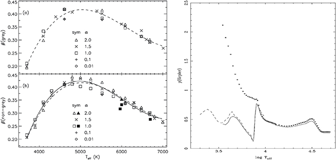
Figure 5.1. Gravity-darkening coefficient β dependence on temperature for
convective envelopes. Left: results for gray (i.e., continuum opacity) and nongray
(i.e., line-blanketed opacity) Uppsala model atmospheres computed by Alencar &
Vaz (1997). Symbols
correspond to different convection efficiency coefficients  . Right: dependence of the gravity-darkening coefficient on
temperature for the Kepler passband (Claret & Bloemen 2011). The solid line
corresponds to Equation (5.5) fit to Kurucz model atmospheres, the
dashed line is a fit to Phoenix model atmospheres, and asterisks correspond to
Martynov's simplified equation fit to Kurucz model atmospheres. Credit: Alencar
& Vaz, A&A, 326, 257, 1997, reproduced with permission © ESO. Credit: Claret
and Bloemen, A&A, 529, 529, A75, 2011, reproduced with permission © ESO.
. Right: dependence of the gravity-darkening coefficient on
temperature for the Kepler passband (Claret & Bloemen 2011). The solid line
corresponds to Equation (5.5) fit to Kurucz model atmospheres, the
dashed line is a fit to Phoenix model atmospheres, and asterisks correspond to
Martynov's simplified equation fit to Kurucz model atmospheres. Credit: Alencar
& Vaz, A&A, 326, 257, 1997, reproduced with permission © ESO. Credit: Claret
and Bloemen, A&A, 529, 529, A75, 2011, reproduced with permission © ESO.
Download figure:
Standard image High-resolution imageSince the gravity-darkening effect depends on the circumstances in stellar envelopes,
it is related not only to the atmospheric parameters ( and
and  ) but also to the internal stellar structure and rotation properties.
This was pointed out by Claret (1999), who introduced the computation of gravity-darkening coefficients into
the stellar evolution code. Statistical studies based on this new formalism (Claret
2000, Figure 1 therein)
yielded a more accurate theoretical prediction for stellar envelopes where both
radiation and convection contribute significantly to energy transfer.
) but also to the internal stellar structure and rotation properties.
This was pointed out by Claret (1999), who introduced the computation of gravity-darkening coefficients into
the stellar evolution code. Statistical studies based on this new formalism (Claret
2000, Figure 1 therein)
yielded a more accurate theoretical prediction for stellar envelopes where both
radiation and convection contribute significantly to energy transfer.
The gravity-darkening correction given by Equation (5.4) is bolometric. Thus, to apply gravity darkening appropriately to passband data, a bolometric correction needs to be made. Such a correction has been first proposed by Martynov (1973) and later expanded by Bloemen et al. (2011) to the following form:

The right panel of Figure 5.1 depicts the dependence of β on temperature for the Kepler passband (Claret & Bloemen 2011).
Espinosa Lara & Rieutord (2011) also pointed out the failure of von Zeipel's theorem for rapidly rotating stars. They proposed a model that describes latitudinal variation of gravity darkening as a consequence of rotation. In their subsequent paper, Espinosa Lara & Rieutord (2012) further developed the formalism for gravity darkening in binary stars and advocated for the abandonment of a single-parameter description and replacing it with the following expression:

where f(x, y,
z) is surface flux at point (x, y,
z),  ,
,  is the effective gravitational acceleration, and geff is the magnitude of
  . This integral can be solved numerically to obtain a relationship
between the flux and gravitational acceleration.
. This integral can be solved numerically to obtain a relationship
between the flux and gravitational acceleration.
5.2. Reflection Effect
When components in a binary system are close, i.e., when their radii are ∼ 15%–20% of their separation or more (Wilson 1990), surface irradiation of one component by the other becomes important. A part of the incident flux heats the surface of the irradiated star, increasing the temperature, and the other part of the incident flux is reflected off the irradiated star. This effect is called the reflection effect.
Before we develop the formalism to account for the reflection effect, we should identify the cases where reflection contributes significantly to the overall flux of the irradiated component. There are indeed quite a number of such cases, ranging from stars similar in size and effective temperature (Hilditch et al. 1996), to cataclysmic and pre-cataclysmic binaries (Pigulski & Michalska 2002), to rapidly rotating Algols (Olson & Etzel 1994), to elliptical ellipsoidal variables known as heartbeat stars (Welsh et al. 2011).
The rigorous treatment of the reflection effect in binary stars was first developed by Wilson (1990); before that work only approximate solutions existed—see a thorough review by Vaz (1985) on this topic.
Consider a close binary as depicted in Figure 5.2. To properly account for the heating of a
given surface element dA1 on the primary star, we need to sum all contributions to irradiation over
all surface elements dA2 on the secondary star. Following the energy conservation principle, recall
that heating is a bolometric process, whereas radiation is wavelength dependent,
described by the spectral energy distribution (SED) function (blackbody, model
atmospheres, ...). Bolometric emergent intensity  emitted from surface element dA2 into the direction of dA1 may be expressed as the limb-darkened normal bolometric emergent intensity
  :
:

where  is the cosine of the angle between the surface normal to
dA2 and the direction
is the cosine of the angle between the surface normal to
dA2 and the direction  that connects the two surface elements. The incident intrinsic flux
from dA2 to dA1 can then be written per Equation (4.15) as:
that connects the two surface elements. The incident intrinsic flux
from dA2 to dA1 can then be written per Equation (4.15) as:

where  is the cosine of the incident angle between the surface normal to
dA1 and the direction
is the cosine of the incident angle between the surface normal to
dA1 and the direction  .
.

Figure 5.2. Irradiation of the primary star (left) by the secondary star (right). To properly
account for the heating of the surface element  on the primary star, contributions to irradiation of all surface
elements
on the primary star, contributions to irradiation of all surface
elements  on the secondary star must be summed up. Angle
  is the angle between the surface normal
  and the direction
  connecting the two surface elements. Its counterpart
  is not depicted for decluttering purposes. Angles
  and
and  between
  and
and  are also not depicted.
Download figure:
Standard image High-resolution imageWe now introduce a reflection factor  as the ratio of the total (intrinsic + reflected) flux to intrinsic
flux. If there is no reflection,
as the ratio of the total (intrinsic + reflected) flux to intrinsic
flux. If there is no reflection,  . The total incident flux from dA2 to dA1 can then be computed by multiplying the intrinsic incident flux, given by
Equation (5.8), by
. The total incident flux from dA2 to dA1 can then be computed by multiplying the intrinsic incident flux, given by
Equation (5.8), by  2:
2:

where we used the visibility function  defined by Equation (4.13), this time pertaining to the visibility of
surface elements along the line s.
defined by Equation (4.13), this time pertaining to the visibility of
surface elements along the line s.
A fraction of the total incident flux will be used for heating the irradiated surface,
and a fraction will be reflected. The two fractions need to sum up to 1, and they are
determined by the bolometric albedo of the star,  . It is the ratio of the reradiated flux to irradiated flux. Thus, the
fraction of reflected flux is given by:
. It is the ratio of the reradiated flux to irradiated flux. Thus, the
fraction of reflected flux is given by:

The intrinsic bolometric normal emergent intensity  emitted from the surface element dA1 is computed from the polar emergent intensity
  corrected for gravity darkening via Equation (5.4). Note that
Equation (5.4)
relates fluxes and not intensities, but as these are bolometric intensities (integrated
over all wavelengths), it means that
corrected for gravity darkening via Equation (5.4). Note that
Equation (5.4)
relates fluxes and not intensities, but as these are bolometric intensities (integrated
over all wavelengths), it means that  per Stefan–Boltzmann's law, irrespective of the actual distribution of
I(λ). In other words, all models
for I(λ) (blackbody, Kurucz, ...), when integrated over
all λ, must yield
per Stefan–Boltzmann's law, irrespective of the actual distribution of
I(λ). In other words, all models
for I(λ) (blackbody, Kurucz, ...), when integrated over
all λ, must yield  .
.
The intrinsic bolometric flux  is computed per Equation (4.5):

The ratio  is easily related to the reflection factor
  :
:

Similarly, for the other star,

Equations (5.9), (5.10), and (5.12) thus form a recursive set to compute  , and their counterparts for the secondary star form a recursive set to
compute
, and their counterparts for the secondary star form a recursive set to
compute  . In practice, this means that we start from some initial values for
  and
and  , say, unity, and then iterate the recursion set until we reach a
desired accuracy.
, say, unity, and then iterate the recursion set until we reach a
desired accuracy.
Once the converged values of  and
and  are computed, we can calculate a new effective temperature of the
surface element that encompasses the radiation of both intrinsic and reflected
energy:
are computed, we can calculate a new effective temperature of the
surface element that encompasses the radiation of both intrinsic and reflected
energy:

We can do this only because all quantities that partake in reflection are bolometric.
The above procedure may be repeated iteratively any number of times to accommodate for multiple reflections: the total emergent flux from the primary star now heats the secondary star by an amount greater than what the intrinsic emergent flux by itself would cause.
A keen eye will catch that this description neglects the fraction of the incident flux that is not reflected. This may or may not be a problem: if we assume that the absorbed energy is redistributed across the entire star, the effect will not be significant. However, if we assume that the absorbed energy is localized to the immediate vicinity of the irradiated area, then we expect an additional local temperature increase. This was first worked out by Prša et al. (2016). The basic difference in the treatment is the energy balance equation (see Figure 5.3):


where  is the radiosity operator that describes the physical
process of heating and reflection/scattering. The two simplest processes are Lambertian,
described by
is the radiosity operator that describes the physical
process of heating and reflection/scattering. The two simplest processes are Lambertian,
described by  , and limb-darkened distribution, described by
  . An expanded reflection theory has been developed by Horvat et al.
(2018), which includes
different energy redistribution modes: local, latitudinal, and global (Figure 5.4). Their approach further
generalizes the treatment of reflection, but it comes at a significantly higher
computational cost.
. An expanded reflection theory has been developed by Horvat et al.
(2018), which includes
different energy redistribution modes: local, latitudinal, and global (Figure 5.4). Their approach further
generalizes the treatment of reflection, but it comes at a significantly higher
computational cost.
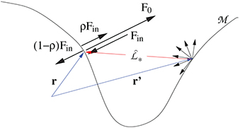
Figure 5.3. Schematic representing the energy balance given the total irradiation of the
element at  . Fin is the total incident bolometric flux,
  is the fraction of Fin that is reflected,
  is the fraction of Fin that is absorbed, and
  is the radiosity operator that describes the physical process of
heating and reflection/scattering. The total emergent flux is denoted with
F0.
is the radiosity operator that describes the physical process of
heating and reflection/scattering. The total emergent flux is denoted with
F0.
Download figure:
Standard image High-resolution image
Figure 5.4. Local (left) and latitudinal (right) redistribution of energy being absorbed at the surface element depicted in black and emitted from the surface areas depicted in red. The regions depicted in yellow represent the area affected by redistribution. Adopted from Horvat et al. (2018).
Download figure:
Standard image High-resolution image5.3. Stellar Spots
The discovery of chromospheric activity of the Sun dates back to prehistoric times (ancient China and ancient Greece), but it was not until Galileo & Harriot observed them in 1610 and until Fabricius published his observations in 1611 that the world truly embraced the concept of sunspots, challenging the perfect, unchanging nature of the universe. Proposing spots on other stars followed shortly, by Boulliau (1667), but we had to wait for actual observations of spots until Kron (1947), who observed eclipsing binary AR Lac and invoked starspots to explain aperiodic out-of-eclipse variability. Over the next several decades we learned that starspots are connected to stellar magnetic fields (Spruit & Weiss 1986), so we expect most (if not all) convective envelope stars to feature spots. Another type of spot is related to mass transfer and accretion in cataclysmic variables (Warner 2003), which are hotter and brighter than the underlying photosphere. A comprehensive review of our current understanding of starspots is given by Strassmeier (2009).
Modern observations of starspots abound; Figure 5.5 depicts a light curve of KIC 2438502, an eclipsing binary with an 8.36-day period that features an RS CVn-type component that rotates with a period of ∼8.23 days. Most out-of-eclipse variation in this light curve originates in chromospheric activity, which is not periodic; hence, it results in the smearing of the phased light curve. Starspot evolution of two persistent active longitudes for this object has been reported and studied by Roettenbacher et al. (2016).

Figure 5.5. Kepler light curve of KIC 2438502, an RS CVn-type eclipsing binary star. The dominant variations are a consequence of chromospheric activity. The time series (left) and phased light curve (right) show that spot activity is neither periodic nor commensurate with the orbital period of the binary.
Download figure:
Standard image High-resolution imageIn terms of modeling, spots may be described by four parameters:
- SPOT COLATITUDE
 : the colatitude of the spot on the stellar surface, described in
the same coordinate system as the star itself.
: the colatitude of the spot on the stellar surface, described in
the same coordinate system as the star itself. - SPOT LONGITUDE: the longitude of the spot on the stellar surface, described in
the same coordinate system as the star itself.
- SPOT ANGULAR RADIUS: angular size of the spot, usually given in radians.
- SPOT TEMPERATURE FACTOR: the ratio between the temperature of the spot and the local
temperature of the underlying photosphere. Values correspond to hot spots, while values correspond to cool spots.


The key assumption when modeling the area covered by a spot is that its local temperature is modified by the temperature factor and the area then radiates as if it were a normal photosphere at that modified temperature.
We can justly question the adequacy of this simplistic description: to properly model spots, advanced and reliable methods of data acquisition (polarimetry, Doppler tomography) are required (see chapter 2). It is not straightforward to use the data in the sophisticated treatment of spots (e.g., nonuniform spot brightness, magnetohydrodynamic effects, etc.), especially as introducing spots without clear support by the data may easily reproduce any physical effect—the degeneracy is typically severe. Even such a simplified treatment, along with any temporal evolution of spot parameters, is thus still ahead of the majority of our current observational capabilities.
5.4. Doppler Boosting
The amount of light that reaches the observer is affected by the kinematic properties
of the radiating body. There are three important velocity-induced changes to the
received flux: (1) Doppler shift of the spectrum causes the passband-weighted integral
to change (Equations (4.27) and (4.28)); (2) Doppler shift of the frequency causes the arrival rate of the
photons to change because of time dilation; and (3) relativistic beaming, where
radiation is no longer isotropic but becomes direction-dependent because of light
aberration (Rybicki & Lightman 1979, chap. 4.8). Loeb & Gaudi (2003) showed that the
boosting signal in exoplanet-hosting stars is larger than variability due to reflected
light from the planet; Zucker et al. (2007) performed a similar study for binary
stars and showed that ellipsoidal variability, reflection, and boosting are
same-order-of-magnitude effects in binaries with a  -day orbital period, while boosting dominates in binaries with a
  -day orbital period. Studies by van Kerkwijk et al. (2010) and Bloemen et al.
(2011, 2012) apply this correction to
Kepler objects KOI-74, KOI-81, and KPD 1946+4340 and demonstrate that
the contributions of boosting are indeed crucial to model the light curves
correctly.
-day orbital period. Studies by van Kerkwijk et al. (2010) and Bloemen et al.
(2011, 2012) apply this correction to
Kepler objects KOI-74, KOI-81, and KPD 1946+4340 and demonstrate that
the contributions of boosting are indeed crucial to model the light curves
correctly.
The combined Doppler boosting signal can be written as:

where Iλ
is the boosted passband intensity, I0, λ
is the initial passband intensity, vr
is the radial velocity, c is the speed of light, and  is the boosting index,

where  is the spectral index, and 5 comes from the Lorenz invariance of
Iλ5 (Loeb & Gaudi 2003). Figure 5.6
depicts the boosting index for the broad Johnson V passband, for a
series of
is the spectral index, and 5 comes from the Lorenz invariance of
Iλ5 (Loeb & Gaudi 2003). Figure 5.6
depicts the boosting index for the broad Johnson V passband, for a
series of  K,
K,  , [M/H] = 0.0 spectra where μ ranges from 0.001 to
1.0. The dependence of the boosting index on wavelength is notable, but in the
simplified approach we approximate the monochromatic boosting factor
, [M/H] = 0.0 spectra where μ ranges from 0.001 to
1.0. The dependence of the boosting index on wavelength is notable, but in the
simplified approach we approximate the monochromatic boosting factor  with the passband-averaged value:

(or its photon-weighted counterpart per Equation (4.28)). This is done
by fitting a Legendre polynomial of the fifth order to the  data; the order is determined by evaluating the rank of the
coefficient matrix in the least-squares fit and seeing where the values become
susceptible to numerical noise. The series was fit iteratively, as data points that lie
below the −1σ threshold were discarded by sigma-clipping the data set.
The iteration stopped when no further points are removed. Another benefit of Legendre
polynomials is their analytical derivative; this analytic form is used to derive the
average boosting index for every model atmosphere. Figure 5.6 also shows that the dependence of the
boosting index on μ is significant, so the traditional approach of
using integrated flux SEDs to estimate
data; the order is determined by evaluating the rank of the
coefficient matrix in the least-squares fit and seeing where the values become
susceptible to numerical noise. The series was fit iteratively, as data points that lie
below the −1σ threshold were discarded by sigma-clipping the data set.
The iteration stopped when no further points are removed. Another benefit of Legendre
polynomials is their analytical derivative; this analytic form is used to derive the
average boosting index for every model atmosphere. Figure 5.6 also shows that the dependence of the
boosting index on μ is significant, so the traditional approach of
using integrated flux SEDs to estimate  is less precise than the treatment presented here.

Figure 5.6. Boosting index  for the Johnson V broadband filter. The spectra
correspond to
for the Johnson V broadband filter. The spectra
correspond to  K,
K,  , [M/H] = 0.0, and μ runs over 33 values ranging
from 0.001 to 1.0. The dependence of the boosting index on wavelength is obvious,
but at this time we approximate it with a weighted average across the passband (see
Equation (5.19)). The increased curviness at larger μ is due to the
larger variations and larger fluxes as we look toward the center of the stellar
disk. Taken from Prša et al. (2016). © 2016. The American Astronomical
Society.
, [M/H] = 0.0, and μ runs over 33 values ranging
from 0.001 to 1.0. The dependence of the boosting index on wavelength is obvious,
but at this time we approximate it with a weighted average across the passband (see
Equation (5.19)). The increased curviness at larger μ is due to the
larger variations and larger fluxes as we look toward the center of the stellar
disk. Taken from Prša et al. (2016). © 2016. The American Astronomical
Society.
Download figure:
Standard image High-resolution imageBoosting is a significant effect, and it becomes a dominant effect over ellipsoidal variation and reflection for longer-period systems. Figure 5.7 shows a comparison of the amplitude of ellipsoidal variation (blue), reflection (green), and Doppler boosting (red) as a function of orbital period for an A0–K0 main-sequence pair in the Johnson V passband (Prša et al. 2016). Ellipsoidal variation and reflection dominate the short-period end, with boosting taking over at around 8 days. Figure 5.8 depicts a light curve with no effects computed (black), with only ellipsoidal variations (blue), with ellipsoidal variations and reflection (green), and with ellipsoidal variations, reflection, and boosting (red).
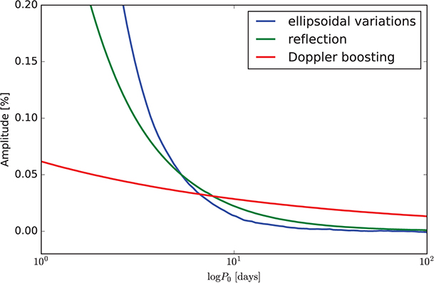
Figure 5.7. Amplitudes of ellipsoidal variation (blue), reflection (green), and boosting (red)
for an A0–K0 main-sequence pair in the Johnson V passband as a
function of orbital period. The semimajor axis is constrained to conserve the masses
of components. For this particular system, ellipsoidal variations dominate the
short-period end, reflection takes over at  days, and boosting takes over at
  days. Taken from Prša et al. (2016). © 2016. The American Astronomical
Society.
days. Taken from Prša et al. (2016). © 2016. The American Astronomical
Society.
Download figure:
Standard image High-resolution image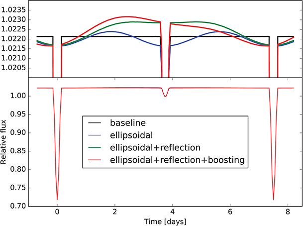
Figure 5.8. Light curve of an A0–K0 main-sequence pair in a 7.5-day orbit. The top panel is the zoomed-in version of the bottom panel. Four models are being plotted: the baseline model (black), which assumes spherical stars; the ellipsoidal variation model (blue), which includes surface deformation due to tides and rotation; the ellipsoidal variation model with reflection (green), which introduces reflection; and the complete model (red), which accounts for Doppler boosting on top of other effects. While the effects are small in amplitude as evident from the bottom panel, high-precision (mmag or better) photometry will routinely demonstrate these effects. Adopted from Prša et al. 2016 © 2016. The American Astronomical Society.
Download figure:
Standard image High-resolution image5.5. Interstellar and Atmospheric Extinction
Interstellar extinction is an extrinsic effect that causes a wavelength-dependent reduction of light that reaches the observer. It was first reported by Trumpler (1930) and connected with dust grains that form the interstellar medium. Extinction is also known as reddening because it affects the blue part of the spectrum more than the red, making objects appear redder than they are intrinsically (Draine 2003). It is usually described by the color excess:

It provides a measure of reddening in terms of the B − V color index change. The slope of the extinction curve in the optical part of the spectrum is given by:

where AB
and AV
are extinctions (in mag) in the B and V
passbands, respectively. The value of RV
depends on the grain size. For example, Rayleigh scattering similar to that in
our atmosphere ( ) would produce a slope of RV
∼ 1.2; extinction in our Galaxy ranges between ∼2 and ∼6, with an average around
RV
∼ 3.1. The larger the grain size, the larger the RV
; in the limit of very large grain sizes,
) would produce a slope of RV
∼ 1.2; extinction in our Galaxy ranges between ∼2 and ∼6, with an average around
RV
∼ 3.1. The larger the grain size, the larger the RV
; in the limit of very large grain sizes,  (Draine 2003). This regime is called gray extinction, i.e., extinction does not depend
on the wavelength.
(Draine 2003). This regime is called gray extinction, i.e., extinction does not depend
on the wavelength.
The most frequently used model to describe wavelength dependence of interstellar extinction is that of Cardelli et al. (1989). It is an empirical formula with the assumed extinction slope RV = 3.1. The formula is split into three wavelength regions:
| Region | λ-interval |
 -interval -interval |
| UV |
|
|
| Optical/NIR |
|
|
| IR |
|
|
The amount of interstellar extinction at a given wavelength (see Figure 5.9) is described by the interpolation formula:

where A(λ) is extinction in mag at the
given wavelength, expressed relative to the visual extinction AV
; x = 1/λ is given in  . Coefficients a(x) and
b(x) are computed by the following
expressions:
. Coefficients a(x) and
b(x) are computed by the following
expressions:
| Region | |
|---|---|
| UV |
![$a{(x)=1.752-0.316x-0.104/[(x-4.67)}^{2}+0.341]-0.04473{(x-5.9)}^{2}\,-\,0.009779{(x-5.9)}^{3}$](https://content.cld.iop.org/books/10__1088_978-0-7503-1287-5/revision2/bk978-0-7503-1287-5ch5ieqn41.gif)
|
![$b{(x)=-3.090+1.825x+1.206/[(x-4.62)}^{2}+0.263]+0.2130{(x-5.9)}^{2}\,+\,0.1207{(x-5.9)}^{3}$](https://content.cld.iop.org/books/10__1088_978-0-7503-1287-5/revision2/bk978-0-7503-1287-5ch5ieqn42.gif)
|
|
| Optical/NIR |

|

|
|

|
|
| IR |
|
|
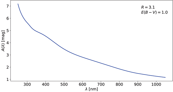
Figure 5.9. Reddening model of Cardelli et al. (1989). Visual extinction slope  and color excess
  are assumed.
Download figure:
Standard image High-resolution imageA standard approach used in the literature to deredden the data is to estimate the amount of reddening from extinction tables (e.g., Schlegel et al. 1998; Gonzalez et al. 2013; Green et al. 2018) given an object's equatorial coordinates. The tables provide color excess along the line of sight, which, given RV and distance, can be used to calculate passband extinction A(λ). This extinction is then subtracted from photometric observations. These tables are either 2D (integrated along the line of sight) or 3D (provide color excess as a function of distance). The "ultimate" extinction table is expected to come from ESA's Gaia mission (Schultheis et al. 2015).
There is a significant problem with this standard approach when applied to eclipsing binary stars: as there are two stars that contribute to total flux and their relative contributions change with phase (i.e., ellipsoidal variations, eclipses, spots, etc.), the amount of reddening also changes, and subtracting a single constant introduces systematic trends as a function of phase. The magnitude of these trends increases with the color difference between the components and with the amount of extinction (Prša & Zwitter 2005).
A much more suitable approach to account for interstellar extinction is to multiply the underlying model atmospheres by monochromatic extinction A(λ) and integrate over wavelength:

so Equation (4.27) becomes:

Thus, we can expand the atmosphere lookup tables by adding another dimension, Apb, and interpolate as before to obtain the correct amount of interstellar extinction added to the model (Jones et al. 2018, in preparation).
To demonstrate the effect of reddening on eclipsing binaries, consider a pair of main-sequence stars with temperatures 6500 and 5500 K, orbiting in a circular orbit with an i = 90° inclination. Say we observe such a binary in Johnson B and V passbands. We will correct for extinction in two ways: by using the standard approach and by using the wavelength-dependent approach. We will neglect all other effects (limb darkening, gravity brightening, reflection effect) so that we evaluate solely the impact of reddening.
The logic is as follows: for the given phase, we compute the effective spectrum of the binary by summing the Doppler-shifted spectra of the visible surfaces of both components. To this intrinsic spectrum we apply interstellar extinction as a function of wavelength. We then multiply this reddened spectrum by the instrumental response function (filter transmission × detector response) and integrate over the passband wavelength range to obtain the flux.
For the standard approach we use the same intrinsic spectrum without applying the
wavelength-dependent extinction; instead, we divide the intrinsic spectrum by the
extinction constant and integrate as before. We can then readily compare the two fluxes
as a function of phase. There is a catch, though: as the Cardelli et al. (1989) formula depends on the
wavelength, the extinction constant will also depend on the wavelength. So which
wavelength do we choose? We could naively take the effective wavelength of the passband,
i.e., the wavelength that splits the passband integral into halves. That is not what we
need, though; we need a wavelength that splits the product  into halves. To compute this, we need to repeat the same wavelength
integration process as before just to get a suitable effective wavelength. Table 5.1 summarizes effective
wavelengths computed as a geometric mean of different quantities: passband, reddened
passband, intrinsic spectrum, reddened spectrum, and the "true" composite reddened
spectrum. Clearly, effective wavelength depends strongly on the effective temperature of
the observed object and on the color excess
into halves. To compute this, we need to repeat the same wavelength
integration process as before just to get a suitable effective wavelength. Table 5.1 summarizes effective
wavelengths computed as a geometric mean of different quantities: passband, reddened
passband, intrinsic spectrum, reddened spectrum, and the "true" composite reddened
spectrum. Clearly, effective wavelength depends strongly on the effective temperature of
the observed object and on the color excess  (Figure 5.10). Figure 5.11 depicts the discrepancy between the properly calculated light curve and
the one obtained by subtracting a
(Figure 5.10). Figure 5.11 depicts the discrepancy between the properly calculated light curve and
the one obtained by subtracting a  -calculated constant.
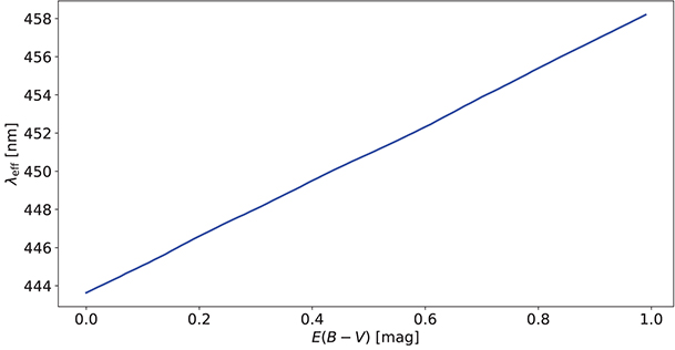
Figure 5.10. Change of the effective wavelength of the Johnson B filter due to reddening of the simulated binary.
Download figure:
Standard image High-resolution image
Figure 5.11. Left: discrepancy due to a simplified constant subtraction approach (blue line)
compared to the rigorously applied reddening (green line) for a model binary. The
subtracted constant was obtained from the effective wavelength ( Å) of the Johnson B transmission curve. Right:
overplotted light curves with the subtraction constant calculated for the
quarter-phase composite reddened spectrum. There is still a measurable difference in
eclipse depth of both light curves.
Å) of the Johnson B transmission curve. Right:
overplotted light curves with the subtraction constant calculated for the
quarter-phase composite reddened spectrum. There is still a measurable difference in
eclipse depth of both light curves.  is assumed.
Download figure:
Standard image High-resolution imageTable 5.1. Summary of Different Approaches to Calculate the Wavelength to Be Used for the Dereddening Constant.
| Approach |

|

|

|
|---|---|---|---|
| Rigorously calculated value | 4470.2 Å | 4.03 | 0.00 |
| Passband transmission | 4410.8 Å | 4.09 | 0.06 |
| Passband transmission + reddening law | 4452.1 Å | 4.05 | 0.02 |
| Intrinsic spectrum | 4436.3 Å | 4.06 | 0.03 |
| Effective (reddened) spectrum | 4583.6 Å | 3.90 | −0.13 |
 is determined by requiring that the area under the spectrum on
both sides is equal.
is determined by requiring that the area under the spectrum on
both sides is equal.  is the value of extinction in the B passband,
and
is the value of extinction in the B passband,
and  is the deviation from the rigorously calculated value. All
values are calculated for
is the deviation from the rigorously calculated value. All
values are calculated for  at quarter phase.
Even if the subtraction constant is properly calculated, the light curves will still exhibit measurable differences in both minima (Figure 5.11). This is because of the color index (effective temperature) dependence on phase, most notably during eclipses. For the case at hand, the difference in B magnitude is ∼1.75 mmag. For the case of a B0V–K4III binary, the same difference inflates to ∼0.2 mag (Prša & Zwitter 2005).
If light curves in three or more photometric passbands are available, it is possible to
uniquely determine the color excess value  by comparing color indices in and out of eclipse. The reddening may
thus be properly introduced as a parameter that can be adjusted during the fitting
process.
by comparing color indices in and out of eclipse. The reddening may
thus be properly introduced as a parameter that can be adjusted during the fitting
process.
Atmospheric extinction is an equivalent but a better-posed problem. As interstellar
extinction depends on  , atmospheric extinction depends on air mass, which (unlike
  ) is a directly measurable quantity. The downside of atmospheric
extinction compared to interstellar extinction is its short-scale time variability: due
to the rapidly changing nature of atmospheric convection cells, the presence of cirrus
clouds, and water vapor, air mass changes unpredictably during the course of
observations.
) is a directly measurable quantity. The downside of atmospheric
extinction compared to interstellar extinction is its short-scale time variability: due
to the rapidly changing nature of atmospheric convection cells, the presence of cirrus
clouds, and water vapor, air mass changes unpredictably during the course of
observations.
To model atmospheric extinction, we use the equation triplet for Rayleigh-ozone-aerosol extinction sources given by Forbes et al. (1996) and summarized by Pakštiene & Solheim (2003):

Rayleigh scattering is given by the following expression:

where P and T are the pressure and temperature during
observations; PSTP = 101,300 Pa and  are the standard temperature and pressure, respectively. Rayleigh
scattering for these standard values is given by:
are the standard temperature and pressure, respectively. Rayleigh
scattering for these standard values is given by:

where λ is the wavelength in  . The formula is normalized to
  , with n being the refractive index and the
coefficient 9.4977 × 10⁻³ corresponding to the optical thickness of the
atmosphere at
, with n being the refractive index and the
coefficient 9.4977 × 10⁻³ corresponding to the optical thickness of the
atmosphere at  . This is adjusted for the height h (in km) of the
observatory above sea level, with the density scale height for the lower troposphere
assumed to be 7.996 km (Forbes et al. 1996). The normalized index of refraction
term may be expressed in terms of wavelength by an empirical relation proposed by
Penndorf (1957):
. This is adjusted for the height h (in km) of the
observatory above sea level, with the density scale height for the lower troposphere
assumed to be 7.996 km (Forbes et al. 1996). The normalized index of refraction
term may be expressed in terms of wavelength by an empirical relation proposed by
Penndorf (1957):

Ozone extinction depends on the amount αozone of ozone in the vertical column of the atmosphere with cross section 1
cm2 and the ozone absorption coefficient  :
:

where 1.1 corresponds to the ozone optical thickness at 320 nm. Values of  are tabulated, e.g., in Cox (2000).
Aerosol scattering on particles with size of the same order of magnitude as the wavelength is the most complicated contribution to the overall atmospheric extinction. It is modeled by the power law:

where A is the extinction at zenith for  and b is the coefficient that depends on the size and
distribution of aerosol particles. These two parameters are very difficult to assess;
fortunately, the aerosol contribution is usually very small, even negligible (Pakštiene
& Solheim 2003). We
neglect its influence in our simulation.
and b is the coefficient that depends on the size and
distribution of aerosol particles. These two parameters are very difficult to assess;
fortunately, the aerosol contribution is usually very small, even negligible (Pakštiene
& Solheim 2003). We
neglect its influence in our simulation.
In terms of binary stars, atmospheric extinction depends on the wavelength of the
observed light and on the air mass of observations, which is of course the same for both
binary components; we are thus left only with wavelength dependence at some inferred air
mass. We can therefore compare the flux change imposed on the intrinsic spectrum by
reddening and by atmospheric extinction (Figure 5.12). For weakly and moderately reddened
eclipsing binaries atmospheric extinction dominates the blue parts of the spectrum owing
to Rayleigh scattering, but for larger color excesses ( ) interstellar extinction is the dominant factor throughout the
spectrum. Since air mass can be measured reliably from observations of comparison stars,
the effect of atmospheric extinction can in principle be removed from the data.
) interstellar extinction is the dominant factor throughout the
spectrum. Since air mass can be measured reliably from observations of comparison stars,
the effect of atmospheric extinction can in principle be removed from the data.

Figure 5.12. Relative flux difference between the intrinsic spectrum and reddened spectrum by  (blue line), by
  (red line), and by atmospheric extinction (green line). The
observatory altitude h = 0 km and the zenith air mass are assumed
throughout the study. If the color excess is large, reddening dominates the
spectrum, but if the color excess is moderate, the blue part of the spectrum is
dominated by the Rayleigh scattering.
(red line), and by atmospheric extinction (green line). The
observatory altitude h = 0 km and the zenith air mass are assumed
throughout the study. If the color excess is large, reddening dominates the
spectrum, but if the color excess is moderate, the blue part of the spectrum is
dominated by the Rayleigh scattering.
Download figure:
Standard image High-resolution image
References
- Alencar S. H. P. and Vaz L. P. R. 1997 A&A 326 257
- Alencar S. H. P., Vaz L. P. R. and Nordlund Å. 1999 A&A 346 556
- Bloemen S., Marsh T. R. and Degroote P. et al 2012 MNRAS 422 2600
- Bloemen S., Marsh T. R. and Østensen R. H. et al 2011 MNRAS 410 1787
- Boulliau I. 1667 Ismaelis Bullialdi Ad astronomos monita duo: Primum, de stella noua, quae in collo Ceti ante annos aliquot visa est Alterum, de neb- ulosa in Andromeda cinguli parte Borea ante biennium iterum orta (Paris: Apud Sebastianum Mabre-Cramoisy)
- Cardelli J. A., Clayton G. C. and Mathis J. S. 1989 ApJ 345 245
- Claret A. 1999 ASP Conf. Ser. 173, Stellar Structure: Theory and Test of Connective Energy Transport , ed A. Gimenez, E. F. Guinan and B. Montesino (San Francisco, CA: ASP) in 277
- Claret A. 2000 A&A 363 1081
- Claret A. and Bloemen S. 2011 A&A 529 A75
- Cox A. N. 2000 Allen's Astrophysical Quantities 4th ed. , ed A. N. Cox (New York: AIP Press)
- Draine B. T. 2003 ARA&A 41 241
- Espinosa Lara F. and Rieutord M. 2011 A&A 533 A43
- Espinosa Lara F. and Rieutord M. 2012 A&A 547 A32
- Fabricius J. 1611 De maculis in sole observatis narration (Wittenberga: ETH-Bibliothek Zürich)
- Forbes M. C., Dodd R. J. and Sullivan D. J. 1996 BaltA 5 281
- Gonzalez O. A., Rejkuba M. and Zoccali M. et al 2013 A&A 552 A110
- Green G. M., Schlafly E. F. and Finkbeiner D. et al 2018 arXiv:1801.03555
- Gustafsson B. 1983 MitAG 60 139
- Hilditch R. W., Harries T. J. and Hill G. 1996 MNRAS 279 1380
- Horvat M., Conroy K. E. and Pablo H. et al 2018 ApJS 237 26
- Kippenhahn R. 1977 A&A 58 267
- Kron G. E. 1947 PASP 59 261
- Loeb A. and Gaudi B. S. 2003 ApJL 588 L117
- Lucy L. B. 1967 ZA 65 89
- Martynov D. 1973 SvPhU 15 786
- Olson E. C. and Etzel P. B. 1994 AJ 108 262
- Pakštiene E. and Solheim J.-E. 2003 BaltA 12 221
- Penndorf R. 1957 JOSA 47 176
- Pigulski A. and Michalska G. 2002 IBVS 5218 1
- Prša A., Conroy K. E. and Horvat M. et al 2016 ApJS 227 29
- Prša A. and Zwitter T. 2005 ESA SP-576: The Three-Dimensional Universe with Gaia , ed C. Turon et al (Paris: Observatoire de Paris-Meudon) in 611
- Rafert J. B. and Twigg L. W. 1980 MNRAS 193 79
- Roettenbacher R. M., Kane S. R., Monnier J. D. and Harmon R. O. 2016 ApJ 832 207
- Rybicki B. G. and Lightman P. A. 1979 Radiative Processes in Astrophysics (New York: Wiley)
- Schlegel D. J., Finkbeiner D. P. and Davis M. 1998 ApJ 500 525
- Schultheis M., Kordopatis G. and Recio-Blanco A. et al 2015 A&A 577 A77
- Spruit H. C. and Weiss A. 1986 A&A 166 167
- Strassmeier K. G. 2009 A&ARv 17 251
- Trumpler R. J. 1930 PASP 42 267
- van Kerkwijk M. H., Rappaport S. A. and Breton R. P. et al 2010 ApJ 715 51
- Vaz L. P. R. 1985 Ap&SS 113 349
- von Zeipel H. 1924 MNRAS 84 665
- Warner B. 2003 Cataclysmic Variable Stars (Cambridge: Cambridge Univ. Press)
- Welsh W. F., Orosz J. A. and Aerts C. et al 2011 ApJS 197 4
- Wilson R. E. 1990 ApJ 356 613
- Zucker S., Mazeh T. and Alexander T. 2007 ApJ 670 1326
Footnotes
- is determined by requiring that the area under the spectrum on
both sides is equal. is the value of extinction in the B passband,
and is the deviation from the rigorously calculated value. All
values are calculated for at quarter phase.