
Abstract
Adaptive 'life-long' learning at the edge and during online task performance is an aspirational goal of artificial intelligence research. Neuromorphic hardware implementing spiking neural networks (SNNs) are particularly attractive in this regard, as their real-time, event-based, local computing paradigm makes them suitable for edge implementations and fast learning. However, the long and iterative learning that characterizes state-of-the-art SNN training is incompatible with the physical nature and real-time operation of neuromorphic hardware. Bi-level learning, such as meta-learning is increasingly used in deep learning to overcome these limitations. In this work, we demonstrate gradient-based meta-learning in SNNs using the surrogate gradient method that approximates the spiking threshold function for gradient estimations. Because surrogate gradients can be made twice differentiable, well-established, and effective second-order gradient meta-learning methods such as model agnostic meta learning (MAML) can be used. We show that SNNs meta-trained using MAML perform comparably to conventional artificial neural networks meta-trained with MAML on event-based meta-datasets. Furthermore, we demonstrate the specific advantages that accrue from meta-learning: fast learning without the requirement of high precision weights or gradients, training-to-learn with quantization and mitigating the effects of approximate synaptic plasticity rules. Our results emphasize how meta-learning techniques can become instrumental for deploying neuromorphic learning technologies on real-world problems.
Export citation and abstract BibTeX RIS
1. Introduction
Rapid adaptation to unfamiliar and ambiguous tasks are hallmarks of cognitive function and long-standing goals of artificial intelligence. Neuromorphic electronic systems inspired by the brain's dynamics and architecture strive to capture its key properties to enable low-power, versatile, and fast information processing [1–3]. Several recent neuromorphic systems are now equipped with on-chip local synaptic plasticity dynamics [4–6]. Such neuromorphic learning machines hold promise to building fast and power-efficient life-learning machines [7].
Spiking neural networks (SNNs) can be modeled as a special case of artificial recurrent neural networks (RNNs) with internal states akin to the long short-term memory (LSTM) [8]. Using a surrogate gradient approach that approximates the spiking threshold function for gradient estimations, SNNs can be trained to match or exceed the accuracy of conventional neural networks on event-based vision, audio, and reinforcement learning tasks [9–14]. Although these methods achieve state-of-the-art accuracy in SNNs, they are not practically realizable on neuromorphic hardware or any other online learning systems, for several reasons: firstly, learning via (stochastic) gradient descent requires data to be sampled in an independent and identically distributed fashion [15]. However, when sensory data is acquired and processed during task performance, data samples are generally correlated, leading to many convergence problems, including catastrophic forgetting [16]. Secondly, many networks use batch sizes larger than one. While networks with a batch size equal to one eventually converge [17], using a smaller batch size means that learning rates must be smaller as well. Smaller learning rates result in smaller weight updates which require memories or buffers that store the weights or weight updates with higher precision, and hence hardware area. Thirdly, surrogate gradient-based SNN training inherits other fundamental issues of deep learning, namely that very large datasets and a large number of iterations are necessary for convergence. The combination of the three problems stated above, i.e. correlated data samples, data inefficiency, and memory requirements hamper the successful deployment of neuromorphic hardware to solve real-world learning problems.
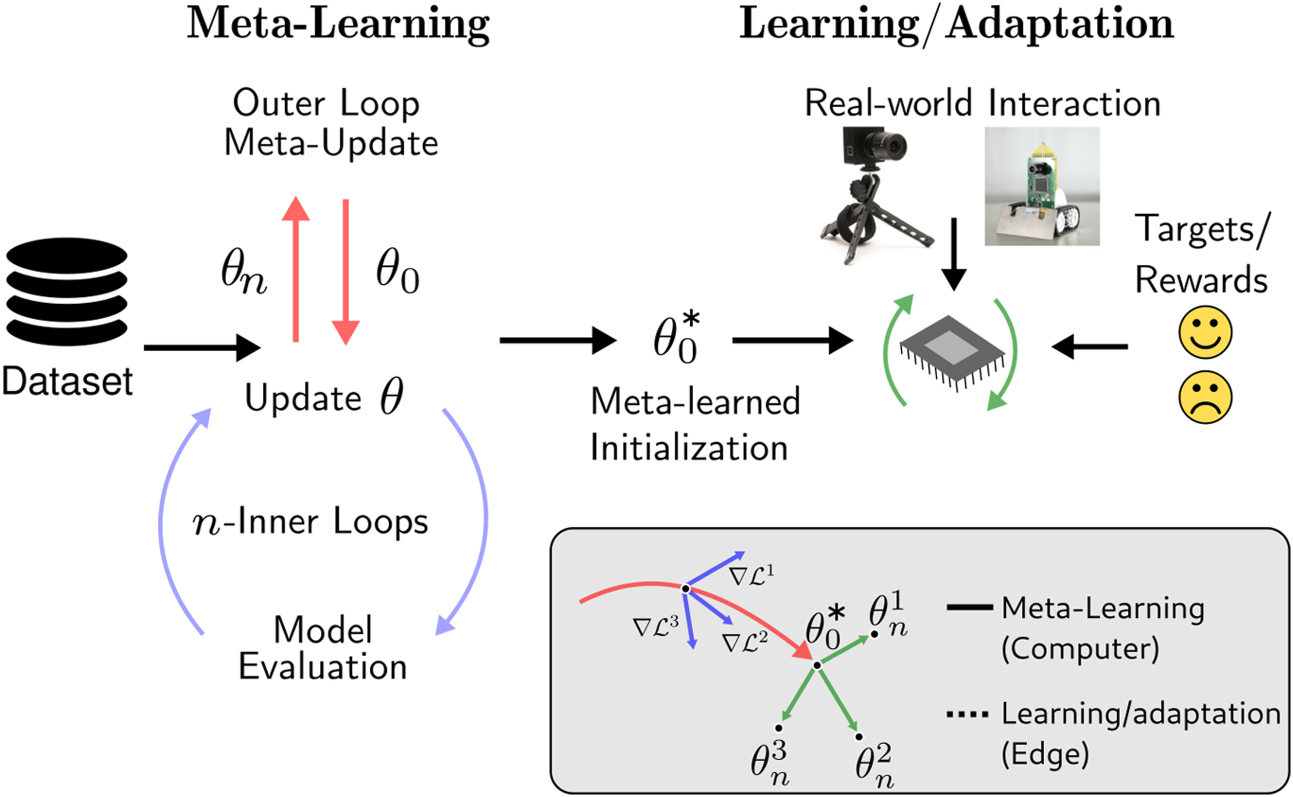
In this article, we demonstrate that gradient-based meta-learning on SNNs can solve these problems in practical cases with technological interest, and are particularly well suited to the constraints of neuromorphic hardware and online learning (figure 1). To do so we combine model agnostic meta learning (MAML), a second-order gradient-based method that optimizes the network hyperparameters, and the surrogate gradient method [8]. Two ingredients were key to the results of our work. First, surrogate functions used to estimate SNN gradients can be made twice differentiable, hence are suitable for second-order learning as in MAML. Second, the definition of suitable event-based datasets to demonstrate meta-learning on SNNs. While MAML had been previously applied to SNNs, prior work focused on meta-training Hebbian spike time dependent plasticity (STDP) dynamics on non-event-based datasets which do not take any advantage of the event-based nature of SNNs [18]. Furthermore, surrogate gradient learning implementing stochastic gradient descent (SGD) can be implemented as a form of three-factor learning [11, 13, 19, 20] that vastly exceeds the performance of classical STDP, while being compatible with neuromorphic hardware implementations [10, 21]. As our results suggest, the meta-training of SNNs using the surrogate gradient method can be used as a tool to adapt and tune synaptic plasticity circuits.

Figure 1. Meta-learning for SNNs using surrogate gradients. In the first phase, an SNN or a functional simulator of a neuromorphic hardware's SNNs is meta-trained using surrogate gradient methods on a class of tasks Ti
stored on a computer. The goal of meta-training is to learn an initial parameter set  such that out-of-sample tasks (e.g.
  ,
,  ,
,  , ...
, ...  ) can be learned quickly. In the envisioned application,
  would be learned offline on a conventional computer and learning/adaption would take place at the edge, using neuromorphic sensing and processing.
Download figure:
Standard image High-resolution imageWe study the SNN MAML approach in the context of few-shot learning, whereby a model is trained on a set of labeled tasks drawn from a given domain of tasks to adapt to unseen ones of the same domain using a small number of samples and iterations. Examples of few-shot learning are learning novel hand or body gestures, agents learning to take new goal-driven actions in a new maze, or optimizing automatic speech recognition to the individual pronunciation of the subject.
One important obstacle to meta-learning research in neuromorphic engineering is the lack of suitable datasets. Neuromorphic hardware implementing SNNs is most suitable to processing event-based datasets and loses most of its salient features when applied to static data [3]. The Omniglot [22] and MiniImagenet [23] datasets have been pivotal in pushing the field of meta-learning ahead. However, there exists no event-based dataset that is comparable to Omniglot or MiniImagenet where modeling dynamics are crucial to solving the problem. The recently published N-Omniglot dataset partially fills this gap [24]. Taking inspiration from existing meta-learning benchmarks that fuse multiple datasets [25], we define new benchmarks that consist of combinations of event-based datasets recorded using neuromorphic vision sensors. We demonstrate performances that are comparable to the performance of conventional neural networks trained on these datasets. We note here that the goal of this work is not to exceed the performance of conventional artificial neural networks (ANNs), but to demonstrate that MAML can successfully be used in the regime corresponding to gradient-descent of SNN dynamics, and thus to fine-tune synaptic plasticity circuits. We demonstrate the latter by training an approximate gradient-based synaptic plasticity rule previously employed in neuromorphic hardware.
Finally, we analyze the updated statistics, which reveal that the MAML not only results in fast learning but does so using large weight updates. These results lay promise for online learning using low-precision weight memory, and are reinforced by meta-learning using differentiable quantization techniques.
1.1. Specific contributions
This work provides (1) a method of parameter initialization that enables neuromorphic hardware to few-shot learn new tasks; (2) a method to construct meta-datasets using data taken from the dynamic vision sensor (DVS) neuromorphic sensor, with two examples made publicly available: double NMNIST, double American sign language dynamic vision sensor (ASL-DVS), N-Omniglot; and (3) the effectiveness of second-order meta-training of SNNs synaptic plasticity rules. This work is thus a stepping stone towards implementing MAML with SNNs in neuromorphic hardware for fast adaptation to streamed event-based sensor data.
2. Methods
2.1. Model agnostic meta-learning
Define a neural network model y = f(x, θ) that produces an output batch y given its parameters θ and an input batch x. For simplicity, we focus here on classification problems, such that y represents logits and argmax y is a class, although any supervised learning problem would be suitable. In the classification case, each batch consists of K samples of each class. The parameters θ are trained by minimizing a task-relevant loss function  , such as cross-entropy, where t is a batch of targets.
The goal of meta-learning is to optimize the meta-parameters of f, such as the initialization parameters noted as θ0. This work makes use of the standard second-order MAML algorithm to meta-train the SNN. The standard MAML workflow is designed to optimize the parameters of a neural network model across multiple tasks in a few-shot setting. MAML achieves this using two nested optimization loops, one 'inner' loop and one 'outer' loop. The inner loop consists of a standard SGD update, where the gradient operations are traced for auto-differentiation [26]. In the outer loop, an update is made using gradient descent on the meta-parameters.
To make use of MAML, it is essential to set up the experimental framework accordingly. Define three sets of meta-tasks: meta training  , meta validation
  , and meta testing
  . Each task T of meta-task
  consists of a training dataset
  and a test dataset
  of the form
  . Here xi
denotes the input data, ti
the target (label) and M is the number of target samples. In general, the datasets corresponding to different tasks can have different sizes, but we omit this in the notation to avoid clutter. During learning, a task is sampled from the training meta-task
. Here xi
denotes the input data, ti
the target (label) and M is the number of target samples. In general, the datasets corresponding to different tasks can have different sizes, but we omit this in the notation to avoid clutter. During learning, a task is sampled from the training meta-task  and N inner loop updates are made using batches of data sampled from
  . The resulting parameters θN
are then used to make the outer loop update using the matching test dataset
. The resulting parameters θN
are then used to make the outer loop update using the matching test dataset  . During each inner loop update, one or more SGD update steps are performed over a task-relevant loss function
  :
:

Here n is the number of inner loop adaptation steps, α is the inner loop learning rate. Note the dependence of θn+1 on the initial parameter set θ0 at the beginning of the inner loop through the recursion.  here indicates the gradient over the inner loop loss
  on the network using parameters θn
. The outer loop loss is defined as:
on the network using parameters θn
. The outer loop loss is defined as:

where  . In practice the above expression is generally computed over a random subset of tasks rather than the full set
  . Notice that the outer loop loss is computed over the test dataset
  , whereas θN
(θ0) is computed using the training dataset
, whereas θN
(θ0) is computed using the training dataset  , which is shown to improve generalization. The goal is to find the optimal θ0, denoted
  such that:

Provided the inner loop loss is at least twice differentiable with respect to θ0, the optimization can be performed via gradient descent over the initial parameters θ0, using a standard gradient-based optimizer using gradients  . Successive applications of the chain rule in the expression above results in second order gradients of the form
  . If these second-order terms are ignored, it is still possible to meta-learn using the method called first-order MAML (FOMAML) [27] and REPTILE [28].
In our experiments, we use the ADAM optimizer for the outer loop loss function and vanilla SGD for the inner loop loss. This choice is motivated by a hybrid learning framework whereby the outer loop training can occur offline with large memory and compute resources (e.g. ADAM which requires more memory and compute), whereas the inner loop is constrained by hardware at the edge. The model is validated and tested on  and
and  , respectively. In the following, we describe the SNN model used with MAML.
2.2. MAML-compatible spiking neuron model
The neuron model used in the SNNs in our work follows leaky integrate & fire dynamics as described in [20]. For completeness, we summarize the dynamics of the neuron model here:

where ui
is the membrane potential, wij
are the synaptic weights between pre-synaptic neuron j and post-synaptic neuron i and Δt is the timestep. Neurons emit a spike  at time t when the threshold of their membrane potential
  is reached.
  is the unit step function, where Θ(ui
) = 0 if ui
< uth
, otherwise 1. p and q describe the traces of the membrane potential of the neuron and the current of the synapse, respectively. For each incoming spike to a neuron, each trace undergoes a jump of height 1 and decays exponentially if no spikes are received. The constants
is the unit step function, where Θ(ui
) = 0 if ui
< uth
, otherwise 1. p and q describe the traces of the membrane potential of the neuron and the current of the synapse, respectively. For each incoming spike to a neuron, each trace undergoes a jump of height 1 and decays exponentially if no spikes are received. The constants

reflect the time constants of the membrane p, synaptic q, and refractory r dynamics. Weighting the trace pj with the synaptic weight wij results in the post-synaptic potential of post-synaptic neuron i caused by pre-synaptic neuron j. The constant bi is a bias current representing the intrinsic excitability of the neuron. The reset mechanism is captured by the dynamics of ri , and the factors τmem, τsyn and τref are time constants of the membrane, synapse, and reset dynamics respectively. Note that equation (4) is equivalent to a discrete-time version of the spike response model with linear filters [29].
To compute the second-order gradients, MAML requires the SNN to be twice differentiable. However, the spiking function Θ is non-differentiable. The surrogate gradient approach, where Θ is replaced by a differentiable surrogate function σ for computing gradients, has been used to successfully side-step this problem [8]. For MAML, the surrogate function can be chosen to be a twice differentiable function. Although many suitable surrogate gradient functions exist, the fast sigmoid function described in [30] strikes a good trade-off between simplicity and effectiveness in learning and is twice differentiable:  . All simulations in this work use the fast sigmoid function as a surrogate function.
Because SNNs is a special case of RNNs, it is possible to apply automatic differentiation tools for implementing the gradient [31, 32]. This also applies to the calculation of the second-order gradients needed for backpropagating the gradient of the inner loss.
2.3. Datasets
We benchmark our models on modifications of datasets collected using event-based vision sensors [33, 34], the neuromorphic MNIST (N-MNIST) [35], and the ASL-DVS [36] datasets. NMNIST consists of 32 × 32, 300 ms long event data streams of MNIST images recorded with an ATIS camera [34]. The dataset contains 60 000 training event streams and 10 000 test event streams. From the N-MNIST dataset, we create double N-MNIST datasets. Each event stream of double N-MNIST is a combination of two N-MNIST event streams to make 64 × 32, 300 ms long event data streams of double-digit numbers that are downsampled to 32 × 16, 100 ms long event data streams. Because there are ten digits in the original N-MNIST dataset, 100 different double-digit numbers can be created. These 100 different numbers can be used to create a meta-dataset with K = 100 tasks, where each double-digit number represents one task. To train and evaluate the performance of meta-trained models we use an N-shot K-way few-shot learning approach. In N-shot K-way learning the model trains on N samples, or shots, of K number of classes, out of all of the available samples and classes in a dataset. The goal of this few-shot learning method is to train models to be able to generalize after seeing as few samples as possible. We create N-shot K-way meta training, meta validation, and meta-test double N-MNIST datasets from the training and test N-MNIST dataset. Each meta dataset consists of a subset of the 100 total possible tasks. The meta training dataset contains 64 classes, the meta validation dataset contains 16 classes, and the meta test dataset contains 20 red classes.
The ASL-DVS dataset contains 24 classes corresponding to letters A–Y, excluding J, in American sign language recorded using a DAVIS 240C event-based sensor [37]. Data recording was performed in an office environment under constant illumination. The dataset contains 4200 240 × 180 100 ms long event data streams of each letter, for a total of 100 800 samples. Like double N-MNIST, each event stream of double ASL-DVS is a combination of two ASL-DVS event data streams to make 480 × 360, 100 ms long event data streams of two letters that are downsampled to 80 × 30, 100 ms long event data streams. Out of the 24 classes, 576 different tasks consisting of double ASL letter event streams can be used to create N-shot K-way meta datasets with each double ASL letter representing a task. From the ASL-DVS dataset, we create double ASL-DVS N-shot K-way meta training, validation, and test datasets. The meta training dataset contains 369 red classes, the meta validation dataset contains 92 red classes, and the meta test dataset contains 115 red classes. Example images from the double N-MNIST and double ASL-DVS datasets are shown in figure 2.

Figure 2. (Top) Examples of double N-MNIST tasks. Each sample contains a combination of two N-MNIST digits to make two-digit numbers. (Bottom) Examples of double ASL-DVS tasks. Each sample contains a combination of two ASL-DVS letters. In all examples, the images are DVS events summed over 100 ms into frames.
Download figure:
Standard image High-resolution imageThe N-Omniglot dataset [24] is a neuromorphic variant of the Omniglot dataset. The original Omniglot dataset contains 1623 categories of handwritten characters, and 20 samples for each category written by Amazon's Mechanical Turk participants [38] and stroke data was recorded. The N-Omniglot leveraged the stroke data to animate writing tracks on a standard 60 Hz display. A DAVIS346 camera was then used to capture these spatiotemporal visual patterns with μs timestamps [24]. The tracks for each character sample lasted several seconds. Both spatial dimensions of the DAVIS346 output was downsampled by a factor 10, resulting in 2 × 34 × 26 dimensional event streams. To reduce the effect of the 60 Hz flicker, we downsampled the timestamp by a factor of 100 000. Since the SNN is simulated on a time step equivalent to 1 ms, this means an acceleration by a factor of 100 with respect to the DAVIS346 operation, because 100 ms of the DAVIS346 is used for 1 time step of the simulated neuron. In comparison, the SNN baseline provided by the authors in [24] used an acceleration factor that was varied between 333 and 1000. We used the same training and validation split as with the Omniglot dataset. Note there is no test dataset in this split.
For all datasets, gradients were truncated beyond the last 30 ms from the end of the sequence. Therefore, not all of the gradients are used across the time sequence for learning. Table 1 shows explorations with a different number of truncation values showing that reducing the number of truncation steps gradually reduced the accuracy, and truncation at the final step did not converge. In table 1 step size refers to the learning rate of the inner loop adaptation. The step size is increased as the truncation is decreased to keep the learning rate constant proportional to the truncation.
Table 1. Effect of truncation of gradients on double NMNIST learning accuracy.
| Truncation | Test accuracy | Step size |
|---|---|---|
| 50 | 98.32% | 1.0 |
| 30 | 98.46% | 1.0 |
| 15 | 98.44% | 2.0 |
| 10 | 97.66% | 3.0 |
| 5 | 98.16% | 6.0 |
| 1 | 34.20% | 15.0 |
| 1 | 29.59% | 30.0 |
Truncation at 30 ms provided the best trade-off between accuracy and memory footprint.
2.4. Model architecture
The architecture for all models trained are similar, consisting of three convolutional layers and a linear output layer. The SNN model architecture used here followed closely existing models for deep continuous local learning [20], and is summarized in table 2. SNN output membrane potentials are encoded into classes by using the output neuron with the highest membrane potential as the classification.
Table 2. SNN MAML network architecture
| Layer | Kernel | NMNIST output | ASL-DVS output | N-Omniglot output |
|---|---|---|---|---|
| Input | 32 × 16 × 2 | 80 × 30 × 2 | 34 × 26 × 2 | |
| 1 | 32c5p0s1 | 32 × 16 × 32 | 80 × 30 × 32 | 34 × 26 × 32 |
| 2 | 2a | 16 × 8 × 32 | 40 × 15 × 32 | 17 × 13 × 32 |
| 3 | 64c5p0s1 | 16 × 8 × 64 | 40 × 15 × 64 | 17 × 13 × 64 |
| 4 | 2a | 8 × 4 × 64 | 20 × 7 × 64 | 8 × 6 × 64 |
| 5 | 128c5p0s1 | 8 × 8 × 128 | 20 × 7 × 128 | 8 × 6 × 128 |
| 6 | 2a | 4 × 2 × 128 | 10 × 3 × 128 | 4 × 3 × 128 |
| Output | — | K= 5 | K= 5 | K= 5 |
aNotation: Ya represents YxY max pooling, XcYpZsS represents X convolution filters ( YxY ) with padding Z and stride S.
3. Results
3.1. Few-shot learning performance on double NMNIST and double ASL tasks
For the double NMNIST and the ASL datasets, we ran five-way one-shot learning experiments on models trained using MAML. The MAML models were meta-trained on the meta training tasks  with the meta validation tasks
  used to compute the loss gradient in the outer loop. The meta-trained models were then tested on the meta-test tasks
  . A summary of our results for each dataset is shown in table 3. The results in table 3 are obtained from averaging the inference performance of a meta-trained model over ten trials on the test datasets (Dtst) of the meta validation and meta test tasks. Each trial has different random batches of data sampled from training tasks
  and validation tasks
  respectively. All experiments only used a single inner loop gradient step (i.e. in MAML N was set to 1). Additionally, we compare the results of the SNNs to equivalent non-spiking models meta-trained with MAML as well as SNNs trained with FOMAML. FOMAML ignores all terms involving the second-order gradients and is thus similar to the joint training of the tasks. This has the advantage of reducing the memory footprint required for learning but is known to reduce the accuracy of the meta-trained model [27]. For the non-spiking models, the input data is first converted from the address event representation to static images by summing the events over the time dimension.
Table 3. One-shot five-way accuracy results. Validation accuracy indicated accuracy over the test datasets (Dtst) in the meta validation set  and test accuracy indicates accuracy on the meta test set
  .
.
| Task | Algorithm | Validation accuracy | Test accuracy |
|---|---|---|---|
| Double N-MNIST | MAML (SNN) | 98.76 ± 1.05% | 98.23 ± 1.12% |
| MAML (CNN) | 99.09 ± 0.53% | 98.35 ± 1.26% | |
| FOMAML (SNN) | 92.59 ± 1.0% | 92.63 ± 0.74% | |
| Double ASL DVS | MAML (SNN) | 95.77 ± 0.88% | 96.04 ± 2.31% |
| MAML (CNN) | 94.93 ± 0.92% | 94.97 ± 1.63% | |
| FOMAML (SNN) | 94.97 ± 1.12% | 94.27 ± 0.6% |
The results show that both spiking and non-spiking MAML achieve one-shot learning performance on the datasets comparable to the state-of-the-art performance shown by non-meta models. The state-of-the-art test accuracy for standard non-meta model training on the NMNIST dataset with SNNs is 99.2 ± 0.02% accuracy [39]. The SNN achieves 98.23 ± 1.12% test accuracy on double NMNIST in a one-shot learning scenario. Our SNN network achieves a test accuracy on the double ASL-DVS dataset of 96.04 ± 2.31%. For both datasets, FOMAML performed significantly worse, highlighting the importance of differentiable surrogate gradients for successful meta-training.
On average MAML on SNNs tend to match or outperform non-spiking MAML on event-based datasets. This is likely because the dynamics of the SNN neurons are well suited for processing and learning the spatio-temporal patterns of the event-based data streams the datasets are composed of.
3.2. One-shot learning on the N-Omniglot dataset
We tested the same model as above on the N-Omniglot dataset [24]. This dataset consists of 1623 categories of characters, each repeated 20 times by a different writer. Stroke data was used to drive a target on a screen, which was recorded by a neuromorphic vision sensor. As in the work published by Li et al, we binned the data samples in space and time (see methods). On the five-way, one-shot task considered here, our MAML SNN outperformed all baselines reported in Li et al (table 4).
Table 4. Comparison of meta-learning methods on the N-Omniglot dataset.
| Algorithm | Time steps | Test accuracy |
|---|---|---|
| MAML (SNN, this work) | 100 | 96.43 ± 0.66% |
| MAML ([24]) | 4 | 77.2 ± 0.4% |
| Siamese net ([24]) | 4 | 73.1 ± 0.6% |
The higher number of time steps is most likely the reason for the increased performance, as our work sees more of the data, however the differences in the network architecture could have influenced our higher performance as well.
3.3. Generalization of learning performance
MAML requires selecting hyper-parameters such as the number of update steps and the learning rates. In real-world scenarios, the input constraints cannot be tightly controlled, leading to potential mismatches with the MAML hyper-parameters. For example, in a real-time gesture learning scenario, the parameter update schedule may not be tightly linked to the time the gesture is presented. Here we study the ability of MAML trained SNNs to generalize across different input conditions.
The ability of MAML to generalize learning performance across its settings, such as the number of steps, has been previously documented for conventional ANNs [41].
Here, we demonstrate that this feature extends to our SNN. Using an SNN MAML network meta-trained on the double NMNIST dataset, we varied the number of gradient steps during inner loop adaptation on test data. The figure 3 shows how changing the number of gradient steps during inner loop adaptation affects the one-shot five-way learning performance on each dataset. On both datasets, as the number of inner loop gradient steps increases the performance increases. Therefore there is a trade-off between the computational overhead of performing multiple gradient steps during one-shot learning and accuracy.
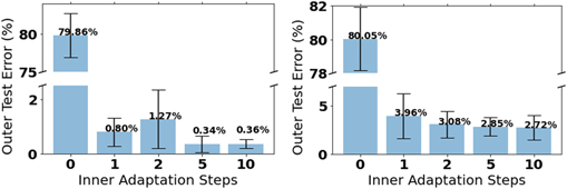
Figure 3. Example of how changing the number of inner loop training steps during meta-testing affects the error of the meta-trained model. Accuracy increases as the number of gradient steps increases and without adapting to a new task the model will have very high error. (Left) Double NMNIST. (Right) Double ASL-DVS.
Download figure:
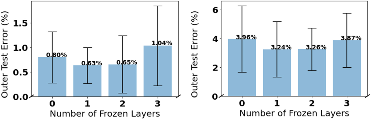
Standard image High-resolution imageWe also show how the learning performance is affected when layers of the network are frozen during few-shot learning. Using a network meta-trained on the double NMNIST dataset, we progressively froze layers of the network to observe the impact on performance, which is shown in figure 4. Even when all layers of the network were frozen, in this case, three, there is not a big impact on performance. This gives further evidence to the claim that MAML learns a suitable representation for few-shot learning instead of rapid learning [40]. This is interesting from an engineering perspective, as the network with a meta-learned initialization can achieve high performance on learning new tasks with only one gradient update and only at the final layer. When all but the last layer are frozen during the inner loop, there is no requirement to backpropagate the errors. This greatly simplifies the learning rule implemented in hardware and is thus suited for real-time adaptation in neuromorphic hardware as demonstrated in previous work [42].

Figure 4. Example of how freezing layers of the network during inner loop adaptation does not greatly impact learning performance. This supports the network is using feature reuse as in [40]. (Left) Double NMNIST. (Right) Double ASL-DVS.
Download figure:
Standard image High-resolution image3.4. MAML few-shot learning relies on few, large magnitude updates
To obtain adequate generalization, conventional deep learning relies on many, small magnitude updates across a large dataset. This is achieved using a relatively small learning rate. The usage of small learning rates is challenging on a physical substrate, as it requires high precision memory to accumulate the gradients across updates. This problem is further compounded by the fact that learning on a physical substrate cannot be easily performed using batches of samples.
Interestingly, few-shot learning has the opposite requirements: few but large magnitude updates. This result is extremely relevant for neuromorphic hardware which uses low precision parameters.
Likewise, we observe that the SNN MAML model only needs a few, large magnitude parameter updates for few-shot learning. The table 5 shows the truncated values of the update magnitude between two training iterations of the output layer for a meta-model and an equivalent non-meta model both trained on double NMNIST. The figure 5 gives a more detailed picture by showing histograms of the weight updates. Comparing the MAML inner loop and the non-meta model's magnitudes, the average update of the inner loop is an order of magnitude larger than the equivalent non-meta model's update. To summarize, we find that, first, meta-trained models only need one adaptation step to achieve high accuracy when learning a new task (see table 3), and second, that these models only need a few updates with a large magnitude to perform few-shot learning (see table 5, figure 5).
Table 5. Comparison of the magnitude of updates between MAML and non-MAML learning.
| Algorithm | Avg. magnitude | Sum of magnitudes | Max. magnitude |
|---|---|---|---|
| MAML outer loop | 7.72 × 10⁻⁵± 0.0002 | 0.296 ± 0.599 | 0.002 ± 0.0017 |
| MAML inner loop | 0.0044 ± 0.0007 | 17.03 ± 2.69 | 0.1548 ± 0.16 |
| Non-meta | 0.0005 ± 0.0002 | 0.5499 ± 0.2412 | 0.0011 ± 0.0002 |
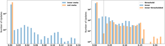
Figure 5. A comparison of the weight update magnitudes on double NMNIST data, shown on a log scale, of an inner loop update and (left) and equivalent not meta trained model update; and (right) an inner loop update that is thresholded. MAML makes fewer non-zero weight updates that are large in magnitude compared to non-meta models. Additionally when thresholded MAML makes fewer non-zero weight updates that are larger in magnitude.
Download figure:
Standard image High-resolution imageAdditionally, the magnitude of the weight updates in the inner loop during meta training and adaptation can be thresholded to use even fewer and larger magnitude updates. During the inner loop adaptation, instead of always updating the parameters the update is gated by a threshold which is described in equation (6)

where  are the parameters of the model, Δw is the magnitude of the update, and Θ is the threshold. Thresholding the updates forces the parameters to be larger with fewer updates, which is shown in the figure 5. The threshold used in the figure 5 was equal to 5% of the value of the range of magnitude updates.
3.5. Comparison to transfer learning
A generalization problem involves learning a function, or model, whose behavior is constrained through a dataset that can make predictions about (i.e. learn features than can transfer to) other samples. A task domain consists of datasets that are related by a common domain, for example, datasets that all consist of double-digit numbers. Learning on one task in the domain to improve performance on another task is commonly referred to as transfer learning. Meta-learning can cast transfer learning as a generalization problem because each example, or task, in a given task domain, is a generalization problem instance in meta-learning, which means generalization in meta-learning corresponds to the ability to transfer knowledge between the different problem instances [43, 44].
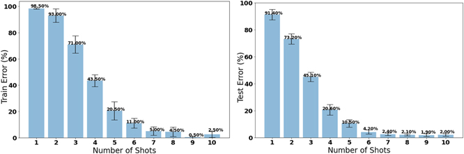
We compare meta-learning to the conventional transfer learning for few-shot learning where a model is pre-trained on a subset of classes within a task domain and then the pre-trained features are transferred to another model that learns to classify new classes within the task domain. For comparison to the double NMNIST SNN MAML model we first pre-trained an SNN model on the 64 classes of the training dataset. Then we transferred the features to a new model that had an untrained last layer. The model was trained and tested on 20 of the remaining classes where all layers except the last layer were frozen. The model was trained on one shot of data at a time and then tested on 20 unseen shots of data. The few-shot transfer learning results are shown in figure 6. The results shown in the table were averaged over ten trials. After the model trains on about nine or ten shots of data, the model achieves comparable accuracy to the SNN MAML model shown in table 3. Comparing that to the high accuracy of the SNN MAML models on new tasks after using only one shot of data (see figure 3, table 3), we can conclude that SNN MAML can adapt to a new task using fewer shots of data.
Figure 6. The error of a pre-trained non-meta model on double NMNIST training classes using transfer learning to learn the test set of classes. The model requires more shots than MAML to achieve comparable performance.
Download figure:
Standard image High-resolution image
3.6. Quantization of parameters during meta-training and meta-testing
The limited availability of memory in neuromorphic devices dictates the necessity for quantization. In most mixed signal and digital CMOS hardware, weights are stored in static RAM in a fixed point format. In the Loihi chip for instances, weights can be programmed to be quantized between 1 bit and 8 bits [6], and updates weights are rounded stochastically [45]. MAML presents an interesting opportunity to meta-train a network with quantization. Furthermore, quantization in the outer loop can be decoupled from the quantization in the inner loop. We have used the following quantization scheme:

where QC,S is a quantization function that updated real-values weights stochastically (S = 1) or deterministically (S = 0). The subscript C refers to allowed levels, which were equally spaced within the interval [−1, 1] and symmetric around 0. Gradients of Q were set to straight through, i.e. ∇x QC,S (w(x)) = ∇x w(x). This quantization scheme makes it compatible with second-order MAML and does not require a copy of real-valued weights during inner loop learning as typically done when quantizing neural networks [46]. The test accuracy on selected configurations of C and S are shown in table 6 with C converted to the bits of precision quantized to. Our explorations revealed that quantization is achievable with a very small loss in performance even when quantized to only 2 bits of precision if stochastic rounding is used for inner loop updates as experimental results show in table 6. However using stochastic rounding in the outer loop for low precisions is detrimental with 6 showing these models do not converge unlike the models that have stochastic rounding in the inner loop at low precisions.
Table 6. MAML SNN quantization experiments. qin: number of bits quantized to in the inner loop, qout: number of bits quantized to in the outer loop, s: stochastic rounding.
| qout | 2 | 2s | 3 | 3s | 4 | 4s | 8 | 8s |
|---|---|---|---|---|---|---|---|---|
| qin | ||||||||
| 2 | 21.6% | 23.8% | 21.3% | 23.2% | 95.7% | 96.3% | 91.4% | 95.9% |
| 2s | 96.7% | N/A | 95.0% | N/A | 83.7% | N/A | 91.5% | N/A |
| 3 | 22.0% | 20.8% | 20.9% | 25.8% | 93.3% | 95.0% | 94.7% | 87.2% |
| 3s | 95.7% | N/A | 91.1% | N/A | 94.2% | N/A | 96.6% | N/A |
| 4 | 92.6% | 81.9% | 98.8% | 56.5% | 99.0% | 97.9% | 98.8% | 99.1% |
| 4s | 97.5% | N/A | 98.2% | N/A | 98.8% | N/A | 97.9% | N/A |
| 8 | 97.5% | 88.3% | 97.0% | 85.6% | 98.5% | 97.8% | 98.9% | 99.2% |
| 8s | 98.6% | N/A | 98.7% | N/A | 97.9% | N/A | 98.5% | N/A |
Furthermore, we found that the quantization in the outer loop is more robust to fewer levels of quantization compared to the inner loop quantization. This interesting fact reveals that MAML can learn a scaffold of network weights on which inner loop synaptic plasticity can learn adequate weights for solving a new task. We speculate that this differential quantization scheme may become useful in hybrid memory designs such as in [47], where initialization weights are stored in precise but area-expensive static RAM, while online weight updates are made in imprecise but power- and area-efficient emerging devices.
3.7. Meta-training with approximations of gradient descent learning rules
Several methods for training SNNs using gradient descent have been introduced. Assuming a global cost function  defined on the spikes s of the top layer, the gradients with respect to the weights are:

The above equation describes a three-factor learning rule [19]. The factor  describes how changing the output in neuron i modifies the global loss and captures the credit assignment problem. Interestingly, this learning rule is compatible with synaptic plasticity in the brain so long as there exists a process that computes (or approximates) and communicates
  to neuron i. Whether and how this can be achieved in a local and biologically plausible fashion is under debate, and there exist several methods to approximate this term on a variety of problems [48]. For instance, direct feedback alignment is an important candidate method to overcome this problem in SNNs [14]. (author?) build on direct feedback alignment by meta-training the random parameters of the feedback alignment.
The relationship of gradient descent with synaptic plasticity means that meta-training is a form of programming of synaptic plasticity. Programming synaptic plasticity is important for mixed-signal neuromorphic hardware implementation of synaptic plasticity because such circuits are prone to mismatch [4, 49]. Even in digital neuromorphic technologies, training programming synaptic plasticity can be useful to approximate an optimal learning rule that would otherwise be impossible or too expensive to implement [6].
To demonstrate the meta-training of a synaptic plasticity rule, we demonstrate MAML on error-triggered synaptic plasticity [21], a variant of equation (8) that has been implemented in the neuromorphic Loihi chip [42] and referred to by the authors as surrogate online error-triggered learning (SOEL)). Error-triggered learning solves two challenges in the implementation of three-factor rules in hardware: continuous-time weight updates which are energy costly and the flexibility necessary to compute  on many types of tasks. It does so by approximating equation (8), namely by triggering a weight update when a neuron's error reaches a threshold value θ:

where ÷ indicates an integer division, and by communicating the resulting positive or negative update across the network. SOEL is a direct adaptation of this rule [42] using the x86 cores in the Loihi chip to estimate Ei
and using a straight-through estimator instead of  to overcome the chip's limitation to two-factor rules. In principle, Ei
can be communicated as an instantaneous rate the neural network. Here we demonstrate that MAML can meta-train a neural network with such a rule, including the estimation of the threshold parameter θ. In this work, we used a floating point division instead of an integer division.
to overcome the chip's limitation to two-factor rules. In principle, Ei
can be communicated as an instantaneous rate the neural network. Here we demonstrate that MAML can meta-train a neural network with such a rule, including the estimation of the threshold parameter θ. In this work, we used a floating point division instead of an integer division.
Table 7 shows the results of meta-training with error-triggered synaptic plasticity on the double N-MNIST, double ASL DVS, and N-Omniglot datasets shown previously without error-triggered synaptic plasticity.
Table 7. One-shot five-way accuracy results with error-triggered synaptic plasticity. Validation accuracy indicated accuracy over the test datasets (Dtst) in the meta validation set  and test accuracy indicates accuracy on the meta test set
  .
.
| Task | Algorithm | Validation accuracy | Test accuracy |
|---|---|---|---|
| Double N-MNIST | MAML SOEL θ = 0.05 | 98.57 ± 1.13% | 98.72 ± 0.20% |
| Double ASL DVS | MAML SOEL θ = 0.05 | 97.81 ± 0.58% | 97.61 ± 0.96% |
| N-Omniglot | MAML SOEL θ = 0.05 | 95.67 ± 2.70% | — |
In all tested cases, the test accuracy of each dataset is comparable to using MAML without the error-triggered rule. Therefore our method adapted from [42] previously used in neuromorphic hardware is suitable for use in neuromorphic hardware.
These results demonstrate that an approximate gradient-based synaptic plasticity rule can be fine-tuned via meta-learning to classification results on par with the exact learning rule. This is particularly interesting for neuromorphic hardware implementations, where exact synaptic plasticity rules are in contradiction with hardware constraints.
4. Discussion
Neuromorphic hardware is particularly well suited for online learning at the edge. Here, we demonstrated how to pre-train SNNs to perform one-shot learning using MAML. The SNN MAML models used the surrogate gradients method to overcome non-linearities that occur in gradient-based training of SNNs. We demonstrated our results on combinations of event-based datasets recorded using a neuromorphic vision sensor.
The effective batch size (=1), the precision required for learning from scratch, and the potential correlation in data samples in neuromorphic learning are serious obstacles to deploying neuromorphic learning in practical scenarios. Fortunately, learning from scratch on the device is generally not even desirable due to robustness and time-to-convergence issues, especially if the devices are intended for edge applications. Some form of offline pre-training can alleviate these issues, and MAML is an excellent tool to automate this pre-training.
Our results showed that a meta-trained SNN MAML model can learn new event-based tasks in one or a few shots within a task domain. This enables learning in real-world scenarios when data is streaming, online, and observed only once. Additionally, the model can relearn prior learned tasks in one or few shots which greatly reduces the impact of catastrophic forgetting because the model does not need to retrain for many iterations.
In hardware for training neural networks, weight updates must be rounded to fall onto values that are resolved at the desired resolution, thereby placing a lower bound to the learning rate. Conveniently, in few-shot learning, updates are of large magnitude (figure 5) and a single update must be sufficient to make a change in the output, effectively implying that the learning rate is large.
Meta-training SNN MAML models require considerable computing power and memory. The tasks are stored in memory as a sequence of length T with network computations calculated over the sequence. Our method re-initializes the network dynamics each iteration of training by inputting a partial sequence of a data sample into the network that executes the dynamics but does not update the network. Additionally, gradients must be computed and stored both in the inner loop and outer loop and backpropagated through the network to meta train. This largely prevents learning for a large number of inner loops. While FOMAML requires less memory and compute for each update, it performed significantly worse than MAML on our model and benchmarks. Other FOMAML methods such as REPTILE [28] are an alternative that can reduce memory usage at the cost of more compute time and some accuracy.
We note that the model agnostic property of MAML renders it complementary to techniques that improve the performance of SNNs, such as batch normalization [50] and dropout [14], or methods to train SNNs such as parameter conversions [51, 52] and neural architecture search [53] such as those applied to SNNs [54]. The latter methods can be directly integrated an additional step in the outer loop update.
4.1. Non-gradient based meta-learning
MAML is known to learn representations that are general across datasets rather than 'learning to learn' [40]. The results of our experiments with freezing model layers showed this is the case for SNN MAML as well indicating the layers already contain good features at meta-initialization. Another meta-learning approach done with artificial RNNs is to train the optimizer itself modeled using an LSTM [43]. The underlying mechanism relies on the recurrent cell states that capture knowledge that is common across the domain of tasks.
The SNN based work [55] falls into this category. There, meta-learning was applied to SNNs trained using e-prop on arm reach and Omniglot tasks. The approach used for the meta-learning combined a learning network to carry out inner loop adaptation and a learning signal generator to carry out outer loop generalization that was both modeled by recurrent SNNs.
4.2. Meta-learning with ANNs
Recent work has given several approaches to achieve high performance on few-shot learning tasks without updating the networks. For example, matching networks [23] utilize two components to enable one-shot learning; a deep neural network augmented with memory, and a training strategy tailored for one-shot learning. The matching network trains an associative memory implemented by an attention mechanism that stores prior information about training data-label pair associations to produce sensible test labels for unobserved classes.
Another salient example is the Siamese network [56], which was more recently applied to one-shot learning [57]. Siamese networks consist of two networks with a common body that learns similarities between the classes of two inputs. By comparing each sample in a small N-way K-shot test set, the Siamese network can be train to distinguish different classes of samples.
Compared to MAML, matching networks and Siamese networks do not require updating the network. However, MAML was shown to outperform matching networks [27] and Siamese networks [24, 27]. Furthermore, the fact that no backpropagation is required with frozen layers and that MAML-based approaches outperform the Siamese net, strongly suggest that matching networks and Siamese networks are less interesting for few-shot learning than our demonstrated approach for neuromorphic hardware.
4.3. Non MAML SNN few-shot learning
MAML and other meta-learning algorithms are not the only methods by which to achieve high accuracy on few-shot learning tasks. Prior work have demonstrated using hybrid SNN-ANN models to achieve high performance on few-shot learning tasks without using MAML. One example is the work of [58] that used a multi time-scale optimization learning to learn approach through the combination of an SNN and an adaptive-gated LSTM trained by BPTT on the Omniglot and DVSGesture [59] datasets. The method enabled using two different timescales for neural dynamics to achieve both short term and long term learning for few-shot learning.
Another example is the work from [60] and their heterogeneous ensemble-based spiking few-shot online learning method that combined an information theoretic approach for training an SNN on features that were extracted from a convolutional ANN on the Omniglot dataset and a robot arm motor control task. Their work achieved accuracy on the Omniglot dataset comparable to ours on the N-Omniglot dataset. Yang et al also demonstrated their method can achieve high performance on noisy data. While both [58, 60] achieve high few-shot learning performance on their datasets, both have ANN components that would not be implementable on neuromorphic hardware. The focus of our work is to lay the foundation for meta-learning with MAML on neuromorphic learning machines.
4.4. Meta-learning for neuromorphic learning machines
The work by [61] developed an online-within-online meta-learning method via meta-gradient descent that is applicable for learning in neuromorphic edge devices without transfer learning. The method uses a three-factor local learning rule that does not use an offline pre-deployment training with backpropagation. This allows a fully online meta learning training method called online-within-online meta-learning for SNNs that performs meta-updates on data streamed to the network. To do the meta updates, multiple SNN models are trained in parallel on the same number of datasets from data sampled by the family of tasks for the outer loop update, and a within-task dataset is used to update an inference SNN in an inner loop update. They evaluated their method on the Omniglot and MNIST-DVS datasets with two-way five shot learning.
[62] showed that plasticity can be optimized by gradient descent, or meta-learned, in large artificial networks with Hebbian plastic connections called differentiable plasticity. Network synapses store both a fixed component, a traditional connection weight, and a plastic component as a Hebbian trace that stores a running average of the product of pre and post-synaptic activity modified by a coefficient to control how plastic the synapse is. Networks using the plastic weights were demonstrated to achieve similar performance to MAML and matching networks. A Hebbian-based hybrid global and local plasticity learning rule similar to the differentiable plasticity presented in [62] was applied with SNNs in the Tianjic hybrid neuromorphic chip [63]. This work meta-optimized Hebbian-based STDP learning rules and local meta-parameters on the Omniglot dataset to examine the performance of the model in few-shot learning tasks on the Tianjic neuromorphic hardware.
Our work extends the one of [63] by directly optimizing a putative three-factor learning rule on event-based data and surrogate gradients that could be used for few-shot learning in neuromorphic hardware. On the surface, our work has similarities with [63], in the sense that it applies meta-learning to SNNs and proposes this method for neuromorphic hardware. However, there are significant algorithmic differences and certain challenges addressed in our work that are not addressed in [63]. Firstly, although not directly stated in [63], their work used a first order method since their surrogate function is not twice differentiable. Secondly [63], uses a Hebbian STDP rule in the inner loop update. However, our work makes use of a gradient descent update, which is equivalent to a three factor synaptic plasticity rule. Third, the datasets used for few-shot learning are not converted from images. Relatedly, their models operates at much coarser time scales (8 time steps for 100 ms, Δt = 12.5 ms), making their model in line with conventional RNNs rather than SNNs. In comparison, the mode of operation in this work uses a time step that is in agreement with existing neuromorphic accelerators (Δt = 1 ms). While Δt = 12.5 ms mode of operation renders the training more tractable for image-based datasets, it does not address a key challenge in neuromorphic processing which is the exploitation of the high temporal precision in event-absed neuromorphic sensors [64, 65].
Meta-learning and transfer learning techniques are already presenting themselves as key tools for neuromorphic learning machines. For example, transfer learning on the Intel Loihi neuromorphic research chip was used to enable few-shot learning [42] There, a gesture classification network was pre-trained using a functional simulator of the Loihi cores. The trained parameters were transferred onto the chip. Using local synaptic plasticity processors, the hardware was able to learn five novel gestures without catastrophic forgetting, achieving 60% accuracy after a single, one second-long presentation of each class. While encouraging, we believe this performance can be improved using our approach utilizing SNN MAML and SOEL.
4.5. Conclusion
We argued that successful meta-learning on SNNs holds promise to help reduce training data iterations at the edge, making it essential to designing and deploying neuromorphic learning machines to real-world problems; prevent catastrophic forgetting and learn with low-precision plasticity mechanisms. As a bi-level learning mechanism, our results point towards a hybrid framework whereby SNNs are pre-trained offline for online learning. As a result, we expect a strong redefinition of synaptic plasticity requirements and exciting new learning applications at the edge.
Acknowledgments
This research was supported by the Intel Corporation (KS, EN), the National Science Foundation (NSF) under Grant 1652159 (EN), NeuroSys as part of the initiative 'Clusters4Future' is funded by the Federal Ministry of Education and Research BMBF (03ZU1106XX), and the Telluride Neuromorphic Cognition Workshop 2020 (NSF OISE 2020624). We would like to thank Jan Finkbeiner for his useful comments.
Data availability statement
The data that support the findings of this study are openly available at the following URL/DOI: https:// github.com/nmi-lab/torchneuromorphic.