

Abstract
Recent studies show that behaviour changes can provide an essential contribution to achieving the Paris climate targets. Existing climate change mitigation scenarios primarily focus on technological change and underrepresent the possible contribution of behaviour change. This paper presents and applies a methodology to decompose the factors contributing to changes in per capita emissions in scenarios. With this approach, we determine the relative contribution to total emissions from changes in activity, the way activities are carried out, the intensity of activities, as well as fuel choice. The decomposition tool breaks down per capita emissions loosely following the Kaya Identity, allowing a comparison between the contributions of technology and consumption changes among regions and between various scenarios. We illustrate the use of the tool by applying it to three previously-published scenarios; a baseline scenario, a scenario with a selection of behaviour changes, and a 2 °C scenario with the same selection of behaviour changes. Within these scenarios, we explore the contribution of technology and consumption changes to total emission changes in the transport and residential sector, for a selection of both developed and developing regions. In doing so, the tool helps identify where specifically (i.e. via consumption or technology factors) different measures play a role in mitigating emissions and expose opportunities for improved representation of behaviour changes in integrated assessment models. This research shows the value of the decomposition tool and how the approach could be flexibly replicated for different global models based on available variables and aims. The application of the tool to previously-published scenarios shows substantial differences in consumption and technology changes from CO2 price and behaviour changes, in transport and residential per capita emissions and between developing and developed regions. Furthermore, the tool's application can highlight opportunities for future scenario development of a more nuanced and heterogeneous representation of behaviour and lifestyle changes in global models.
Export citation and abstract BibTeX RIS

Original content from this work may be used under the terms of the Creative Commons Attribution 4.0 licence. Any further distribution of this work must maintain attribution to the author(s) and the title of the work, journal citation and DOI.
1. Introduction
Model-based scenario studies are often used to explore different strategies to reach climate goals and assess their respective costs and benefits. These studies typically focus on technological options to reduce emissions, including energy efficiency improvement and substitution to supply-side technologies with less or zero greenhouse gas emissions (e.g., renewables and carbon-capture-and-storage) (van Vuuren et al 2018). Only a few global modelling studies explicitly explore the potential role of behaviour measures as mitigation options (IPCC 2014). These studies show that behaviour changes can play a crucial role in reaching long-term climate targets by providing additional options to reduce emissions (van Sluisveld et al 2016, van de Ven et al 2017, Grubler et al 2018, van Vuuren et al 2018, Lettenmeier et al 2019). Nevertheless, the range of behaviour measures in scenarios is limited. For example, energy scenarios do not adequately explore sufficiency (Samadi et al 2017). Thus, a more nuanced approach to behaviour-related scenario development is necessary.
Understanding the role of behaviour change in scenarios can be helpful to understand the possible impact in the future. Behaviour change can reduce emissions by reducing carbon-intensive activities (e.g. travel) or by shifting activities (e.g. from car to public transport). These changes happen alongside technological measures such as energy efficiency improvement (e.g. using more-efficient vehicles) and fuel-switch (e.g. from petrol to electric vehicles).
There are numerous decomposition tools to analyse decarbonisation trends in both historical periods or projections. Many use the Kaya Identity 7 (Kaya and Yokobori 1997) as a basis. Examples in the literature that have applied this to model-based scenarios (Girod et al 2014, Pietzcker et al 2014, Edelenbosch et al 2020) often focus on changes in fuel composition and technology—and do not explicitly look at behaviour changes on a per capita level. Still, showing the possible contribution of behaviour change in future scenarios offers insights into changes in personal consumption patterns and the activities of our everyday lives. It is, therefore, useful to connect to the studies that focused on individual behaviour and that highlight the role of avoiding, shifting and improving (Creutzig et al 2018) climate-related activities. Here avoid refers to an overall reduction of activity levels, shift to an alternative behaviour with lower ecological impact and improve to a different way of performing the same activity (Girod et al 2014, Lettenmeier et al 2019).
This paper expands on the studies above by developing a tool for decomposing factors of emission changes, measuring impact at an individual level, which is linked to the Avoid-Shift-Improve (ASI) framework. More specifically, our research aim is to present a generic decomposition tool for IAM scenarios to analyse the effect of behaviour change vis-à-vis other measures (such as technology change) on both transport and residential per capita emissions. Such an analysis can also provide insights into how IAMs can improve modelling of behaviour changes. This decomposition tool is specifically designed to measure the impact of behaviour measures and not the intent or personal motivations behind them. A different framing is required to conceptualise the intent-orientation of behaviour changes as well as cross-cutting systemic measures (van den Berg et al 2019a).
For the decomposition tool, we adapt the activity, modal share (structure), vehicle intensity and, fuel mix (ASIF) framework for the categorisation of transport emissions (Schipper and Marie-Lilliu 1999) to be more relevant to analyse both transport and residential per capita emissions. We replace the term structure with service for the residential sector. This article will refer to the adapted framework as the activity, structure/service, intensity and fuel mix (ASIF*) decomposition tool. We also align this categorisation with the avoid, shift, improve (ASI) framework (Creutzig et al 2018, van den Berg et al 2019a) to classify behavioural measures. While the critical focus of the paper is on the decomposition tool, we illustrate its use by analysing trends in several existing scenarios for a baseline scenario and two behaviour change scenarios. In the following sections, we first elaborate on the decomposition tool. Second, we apply the tool for a set of previously-developed scenarios for various regions in the transport and residential sectors and third, we discuss the results of the decomposition analyses. Finally, we present our conclusions.
2. Methodology
The ASIF* decomposition tool (see figure 1 and specific details in table 1) distinguishes the contribution of various types of consumption changes and technological changes on changes in per capita emissions. The distinction between these types of changes is essential, as they are characteristically different in several ways. Soft factors, such as habits and social norms, play a more important role in consumption changes than in technology changes. One consumption change factor is activity, which refers to the direct changes in energy demand (e.g. avoiding kilometres or appliances ownership). Another consumption change factor is a change in structure for transport (e.g. shifting transport modes) and service change for residential (e.g. shifting the thermostat temperature), which also represents a change in energy demand. One technology change factor is intensity and refers to the changes in energy use needed for a particular activity (e.g. improving vehicle efficiency). Another technology change factor is fuel mix and refers to the changes in emissions produced per energy used (e.g. improving fuel choice to renewable sources).
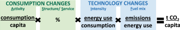
Figure 1. ASIF* factors categorised into contributing factors of consumption and technology changes based on the Kaya Identity, with the corresponding ASI behavioural interventions shown in italics.
Download figure:
Standard image High-resolution imageTable 1. Details of ASIF* factors contributing to per capita emissions.
| Details | ||
|---|---|---|
| ASIF* contributing factors | Transport | Residential |
| Activity | Effects of Changes in transportation demand (i.e. passenger-kilometres (pkm) per capita). | Effects of changes in residential energy demand (e.g. floor space per capita). |
| Structure/service | Effects of Changes in modes of transportation (i.e. pkm per capita in a particular transport mode). | Effects of changes in service demand in residential energy services (e.g. Heating Degree Days, or HDD). |
| Intensity | Effects of Changes in energy intensity within transport modes and fuel type (i.e. energy usage per pkm of a particular transport mode and fuel type). | Effects of changes in energy intensity within residential energy services (e.g. energy usage per HDD of floor space). |
| Fuel mix | Effects of changes in transport fuel types. | Effects of changes in residential fuel types. |
In the literature, there are various types of decomposition analysis for energy and environmental analyses. Ang et al (2003) highlight the strengths and weaknesses of several of these methods. We apply the (Sun 1998) method using the n-term decomposition. Sun's method is a so-called perfect decomposition as it distributes the contribution from interaction terms to their respective factors, leaving zero residual terms. Moreover, contrary to the other conventional methods (like the Laspeyres Index), Sun's method is robust to factor reordering and time-reversal (Ang et al 2003, Ang 2004). The following section explains the application of the decomposition analysis (see figure 2 for the calculation overview in terms of the ASIF* framework).
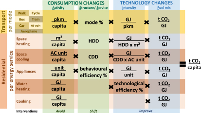
Figure 2. Breakdown of variables and units for decomposition analysis in transport modes and residential energy services in terms of the Activity, Structure/Service, Intensity and Fuel Mix (ASIF*) impact factors HDD = Heating Degree Days, pkm = passenger-kilometre, AC unit = airconditioning unit.
Download figure:
Standard image High-resolution imageThe contributing ASIF* factors to emissions among the sectors transport, residential cooking, residential space heating, space cooling, water heating and appliances is summarised in figure 2. Further details are shown in SI.3. In this ASIF* framework, the CO2 emissions per capita at time t are calculated using an extended version of the Kaya-identity, for each energy service es and region r:

where the fuel mix is calculated by summing over each fuel type f:

The decomposition method used here splits the difference between the per capita CO2 emissions in two years (in our case, 2050 and 2015) in differences attributable to each component:

The exact formulations of each factor of the decomposition are described in SI.2.
The tool decomposes all four ASIF* factors as separate contributors for the energy services transport, space heating, space cooling and appliances. Due to missing representation in the IMAGE model for some factors in water heating and cooking, the tool decomposes three and two factors available (see figure 2). Based on the behaviour measures, these factors would not have a significant impact on the results and can therefore be merged with other factors (see table 3 and more details in SI.3). However, if the decomposition tool would use different scenarios, the methodology should be adjusted to consider these factors explicitly, if relevant.
3. Scenarios analysis
We apply the framework on three scenarios developed by IMAGE (Integrated Model to Assess the Global Environment) to illustrate how the ASIF* framework can help to identify the implications of behaviour change (or other measures, e.g. carbon pricing) in scenarios. The IMAGE 3.0 framework (Stehfest et al 2014) is an integrated assessment model (IAM) to illustrate long-term dynamic changes in the land and energy systems.
Table 2 describes the various previously-published scenarios analysed in this research. The study applies a baseline scenario illustrating a situation in which current trends, including high increases in consumption, are continued without climate policy. This baseline scenario provides a good business-as-usual (BAU) reference to compare with the other scenarios. This research applies a behaviour change scenario to show the effects of behaviour measures such as reduced travel, car use, reduced floor space heated, thermostat adjustments, more efficient use of appliances and shorter shower time (described in table 3). This scenario shows the extent to which the selected behaviour changes contribute to reducing emissions. Furthermore, this study also applies a behaviour change scenario that adopts the behaviour measures in parallel to climate policy measures that align to the Paris climate agreement (limiting average global warming to less than 2 °C Celsius compared to industrial levels). This scenario allows analysis of the added effect of behaviour change under emission reductions forced through carbon pricing.
Table 2. Scenario descriptions.
| Scenarios | Description |
|---|---|
| Baseline scenario | 'Middle-of-the-road' (O'Neill et al 2017) scenario (assumes current social and economic trends and patterns will continue up until 2100, with consumption patterns following GDP per capita trends), without climate policies other than those already implemented. |
| Behaviour change scenario | Behaviour change scenario (van Sluisveld et al 2016) is based on the SSP2 scenario that assumes several behaviour changes within the residential, food and transport sector (e.g. less-meat intensive diet, modal shifts, reduction in heated floorspace and thermostat adjustments; see details in table 3: Overview of implemented behaviour measures for the Behaviour change scenario representing the behavioural actions for various ASIF* factors (adapted from van Sluisveld et al (2016)). |
| Behaviour change + 2 °C scenario | The Behaviour change scenario with climate policies included that aim to stabilise GHG emission concentrations at 450 ppm CO2-eq in 2100, corresponding to a maximum of 2 °C temperature increase in global mean temperature. The emission factor of electricity for some regions becomes negative before 2050 due to extensive use of renewables and bioenergy with carbon capture and storage (BECCS). In our analysis, however, we do not attribute negative emissions to electricity, as otherwise, an increase in demand for electricity would lead, ceteris paribus, to lower emissions per capita. |
Table 3. Overview of implemented behaviour measures for the behaviour change scenario representing the behavioural actions for various ASIF* factors (adapted from van Sluisveld et al (2016)).
| ASIF* factor | Measure | Implementation | Transition | Source | |
|---|---|---|---|---|---|
| Transport | Activity/structure | Reduced vehicle use | Capping the travel money budget (TMB) to not more than 7% of income (compared to the range 6%–10% assumed in the baseline scenario). a | Gradual | van Sluisveld et al (2016) |
| Changing income elasticity to −5% to improve passenger load per mode. | Immediate | Girod et al (2013) | |||
| Structure | Mode shift to public transport | Change of perceived price and increase of daily travelling time budget (TTB) by 0.5 min/year resulting in 122 min/day in 2100 (compared to 0.25 min/year daily TTB increase in the baseline scenario resulting in 97 min/day in 2100). b | Immediate | Girod et al (2013), van Sluisveld et al (2016) | |
| Residential | Service | Reduced heating/cooling demand | Change of base temperature by 1 °C, reducing the number of heating degree days (HDD) or cooling degree days (CDD). | Immediate | Isaac and Van Vuuren (2009), van Sluisveld et al (2016) |
| Activity | Reduced appliance ownership | Reduced ownership levels for 'luxury goods' to zero (e.g. no tumble dryers, dishwashers). | Gradual | van Sluisveld et al (2016) | |
| Maximum ownership rates for other major domestic appliances are fixed to 2013 values. | Immediate | ||||
| Service | More efficient use of appliances | BAT energy consumption estimates and appliances converge to these new levels gradually over time. | Immediate | Goodall (2010) | |
| Activity | Reduced water heating | A correction factor in total energy demand for water heating (based on cutting down 2 min of shower time), based on an estimate in literature. | Immediate | Goodall (2010), Daioglou et al (2012) | |
| Activity | Capping household dimensions | Maximum floor space (m2/cap) is fixed to a representative 2010 value, differentiating for rural (50 m2/cap) and urban households (40 m2/cap). | Immediate | IEA (2004), van Sluisveld et al (2016) |
a Travel money budget (TMB): a travel constraint implemented based on the share of income of the person travelling. b Travel time budget (TTB): a travel constraint implemented based on the time per day spent on transportation.
This study analyses the outcomes for the global average, for the average of a selected set of least-developed regions, and the average of a selected set of highly-developed regions (see SI.1 for the selection of regions). The IMAGE model implements measures and carbon prices similarly and universally across the different regions.
4. Results
In this section, we show the contributions of the ASIF* factors to the change in transport and residential per capita emissions between 2015 and 2050 in the behaviour change scenario and behaviour change 2 °C scenario, compared to the baseline scenario (see scenario descriptions in table 2). In this study, we presented the model responses between two points in time (i.e. 2015 and 2050), but also multiple time steps and thus, trends over time (see figures in SI.4.5 and SI.4.6). The fuel mix (F) is further decomposed into fuel use and emission factors and shown in SI.4.7 for more detail. Refer to SI.4.4 for scenario comparisons including those with exclusively CO2 prices.
4.1. Decomposed transport per capita emissions
In the scenarios analysed, behaviour measures mainly affect global emissions via a mode shift from air and car to trains (S) (see figure 3). There is hardly any change in total pkms (A). This relatively small change can be explained by the underlying assumptions of the behaviour scenario, which consisted of a shift towards Japanese transport patterns via a capped Travel Money Budget (TMB), changed perceived prices and increased Travel Time Budget (TTB) (see table 3). These behaviour measures result in mode-shift but have a small effect on the overall transport distance.
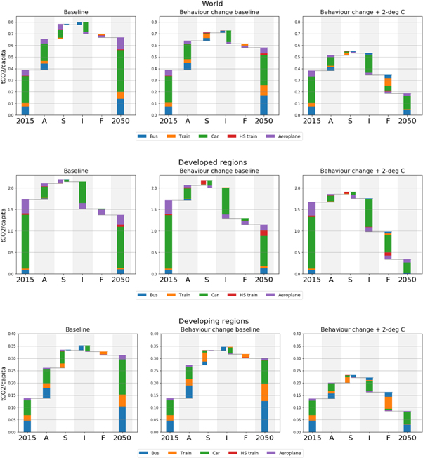
Figure 3. Decomposition of per capita transport emissions for the business-as-usual scenario (Baseline) and two behaviour scenarios that exclude (Behaviour change) and include (Behaviour change + 2-deg) climate policy. The factors A (Activity changes), S (Structural changes), I (Intensity changes) and F (Fuel mix changes) contribute to the change in emissions between 2015 and 2050 for various regions (for more specific regional effects the reader is referred to SI.1).
Download figure:
Standard image High-resolution imageThe behaviour change 2 °C scenario shows the impact of adding a CO2 price in addition to behaviour measures on per capita transport emissions (see SI.4.3. for a scenario comparison with a climate policy scenario). The CO2 price leads to additional reductions in per capita emissions, primarily because of reducing travel demand (A) and changes in the fuel mix (F). The strong impact of changes in the fuel mix on emission reductions is the logical result of the CO2 price changing the relative costs of fuels. The reduction in travel distance is a result of the increase in travel costs. This is consistent with the strong impact of costs on travel demand in IMAGE via the empirically observed fixed TMB. As a result of a carbon tax, it becomes more expensive to travel, consequently resulting in less distance travelled.
There are notable differences in 2015 transport per capita emissions between developing regions and developed regions. As shown in figure 3, developed countries have a factor of 10 higher emissions per capita than developing countries. Almost all emissions in developed countries are from car travel with the remainder from air travel. In contrast, a large portion of the emissions (and thus demand) in developing regions are from buses and trains. There are also contrasting trends between these regions from 2015 to 2050, shown in the baseline scenario. A rapid increase in mobility (A) is projected in the baseline scenario for developing regions along with further development. Developed regions, on the other hand, show high emission reduction from intensity improvements in the baseline scenario in line with historical trends. Compared to the baseline, the behaviour change scenario shows some impacts from mode shifts (S), especially in developing regions. However, for developing regions, the result of mode changes (S) from aeroplane and car to the cheaper train and bus leads to an increase in activity (A).
The inclusion of a CO2 price in addition to the behaviour measures (behaviour +2-deg), results in significant additional improvements in the fuel mix (F). There is also an effect of a CO2 price on the total travel distance (A) in developed regions, but this is relatively small compared to the absolute per capita emission reductions. In contrast, developing regions' emission increase is limited mostly via reduced travel distance (A) and mode shifts (S), and, depending on the scenario, significant improvements in the fuel mix (F). Similar to developed regions, developing regions show high potential for emission reductions by improving the intensity (I) of vehicles/modes and fuel choices (F).
Within the selection of developed regions and developing regions there are notable variations (see the SI.1 for the selection of regions). The characteristics of two developed regions, Japan and the USA (see SI.4.1), differ substantially. The mix of the transport modes is relatively equally distributed in Japan, while in the USA there is a predominant use of car and aeroplane transport modes. For the USA, the highest potential is the reduction of travel distance (A), improvement of intensity (I) and fuel mix (F) in these predominant modes, stimulated mostly by a CO2 price. In Japan, unlike the USA, there is a relatively strong shift (S) to less CO2-intensive transport modes from behaviour measures, with (high-speed) train replacing car and aeroplane travel. The two selected developing regions, India and Western Africa have relatively diverse mixes of transport modes. Thus behaviour measures cause a substantial shift (S) to more sustainable transport modes, especially considering their already low absolute per capita emissions. However, the differences in shift directions are interesting to note. In India, they shift mostly from aeroplane and car to trains, while in Western Africa they shift to buses. Increased train travel in India is logical considering the current proportion of train travel and thus preferences and infrastructure availability. These contrasts between countries highlight how context and situational factors affect behaviour changes, and thus their impacts.
4.2. Decomposed residential per capita emissions
Figure 4 shows the residential per capita emissions that are decomposed for space heating, space cooling, water heating, cooking, and appliances. The trends are markedly different from those of transport. Globally, the behaviour change scenarios, in contrast to transport, shows the considerable impact of activity changes (A) on emissions. Measures likely affecting activity include the capping of floor space heating and reduction of shower time. Changes in energy service demand (S) (e.g. changing thermostat temperatures) have a much lower impact on emissions. Part of this can be explained by higher climate warming in the baseline, resulting in less demand for space heating. The opposite phenomenon occurs in space cooling, as a higher cooling energy demand is needed in a warmer climate – although the effect is relatively small.

Figure 4. Decomposition of per capita residential emissions for the business-as-usual scenario (Baseline) and two behaviour scenarios that exclude (Behaviour) and include (Behaviour + 2-deg) climate policy. The categories A (Activity changes), S (Service changes), I (Intensity changes) and F (Fuel mix changes) represents the contribution of these factors to the change in emissions between 2015 and 2050 for various regions (for regional classification see SI.1).
Download figure:
Standard image High-resolution image
The behaviour change 2 °C scenario shows that with a CO2 price (compared to the behaviour change scenario without a CO2 price the most substantial difference is from the fuel mix improvements (F), and the second-largest difference from activity changes (A) (mostly in appliances). Service changes (S) (e.g. HDD, CDD, use efficiency) have a relatively small effect in both the behaviour change scenario and in the behaviour 2 °C scenario. However, it is vital to note that some energy services do not consider service (S) a separate factor (see figure 2), and thus the service changes (S) refer specifically to the impacts from space heating, space cooling and appliances.
There are substantial differences in 2015 residential per capita emissions between developing regions and developed regions. A notable contrast is that generally-warmer, developing regions tend to have high space cooling. In comparison, generally-colder, developed regions have high heating demand. In contrast to developed regions, developing regions' emissions increase between 2015 and 2050 in the baseline scenario. These increases are attributed mostly due to increased appliance ownership and air conditioners in space cooling, but also some worsening intensity (I) in appliance and space cooling. This latter result is due to additional lower-income households in developing countries gaining access to appliances that have a higher energy consumption (i.e. less-efficient appliances) or have dwellings with poor characteristics for cooling. Furthermore, behaviour measures in the behaviour change scenario have the highest impact via reduced appliance ownership (A). In developed regions, the highest impacts are from reduced floor space heating (A) and from shorter shower times (A) with the corresponding water heating.
We observe some specific differences within the selection of developed regions and developing regions (see SI.1). For example, comparing developed countries USA and Japan (see SI.4.2), a cap on heated floor space has a more considerable emission reduction from activity (A) in the USA which has a relatively larger floor space per capita than Japan. When comparing the two developing regions, India and Western Africa (see SI.4.2), cooking energy demand (A) is a relatively high proportion in Western Africa (but in absolute numbers comparable to India). However, appliance use (A) is a much higher proportion in India. This result is due to the differences in GDP per capita, as the model assumes that higher income leads to more appliance ownership.
5. Discussion
The current study presents the ASIF* decomposition analysis as a tool for IAMs to highlight the impact of behaviour, consumption and technology changes on emissions in scenarios. We applied this tool to decompose per capita emissions in terms of behaviour changes, consumption changes and technology changes. We analysed the effects of carbon pricing and behaviour measures in existing scenarios. This process illustrated how the tool could be used to visualise trends of the impact of consumption and technology changes on emissions and differences in these trends between regions, sectors, and scenarios.
5.1. Expanding the ASIF* decomposition tool
In addition to the model responses between two points in time, we show multiple time steps (as shown in SI.4.5 and SI.4.6). For example, the effect of intensity changes in developed regions is more substantial from 2020 to 2030 compared to the other years. This option of tracking trends is another useful way of interpreting the outcomes of the decomposition tool. It is interesting to explore more ways to present the decomposition outcomes, for example by plotting the decomposition results on an annual basis as pathways instead of a step-wise manner to show more detail on trends over time.
Furthermore, we can expand the tool with additional indicators. For example, the tool could expand water heating, by representing the changes in activity (e.g. reduced shower time) with the unit 'litres per capita'. Furthermore, the tool could represent the service factor as changes in the temperature of water (e.g. less-hot showers). For cooking, The tool could represent the activity as 'kg cooked food per capita' so changes in meal type (e.g. short-cooked meals instead of long-cooked meals) could influence this factor. Within the cooking energy service, a behavioural efficiency (as a percentage) could represent the service (affected by behavioural shifts such as community dinners or batch cooking). Like the other energy services, the intensity represents the changes in technological efficiency as GJ per kg, independent of fuel switches (e.g. more efficient appliances). See SI.6.1 for the proposed structure for decomposition tool of residential and transport emissions. By creating more relevant variables in IAMs, it forms a stronger basis for improved behaviour change, and consequently lifestyle change, modelling for future research.
5.2. Broader application of the decomposition tool
There are other behavioural change scenarios available in the literature (Grubler et al (2018), but applying the decomposition tool is complex given the differences in model outputs. For example, the behaviour change scenario by van Sluisveld et al (2016), analysed in this research, shows significant differences with the LED scenario in a comparable study by Grubler et al (2018) (see SI.5). The former scenario shows lower emission reductions in all sectors compared to Grubler et al (2018)'s LED scenario. For better model response interpretations, it would be valuable to harmonise and compare the results of this decomposition analysis with other scenarios on behavioural change such as the LED scenario (Grubler et al (2018). The ASIF* decomposition tool could function as a basis for harmonisation of various scenarios.
Process-based IAMs with a high spatio-technological resolution (Wilson et al 2017) are considered most suitable to include in a broader application of the ASIF* decomposition tool given their closest representation of consumer behaviour and decision-making. If IAMs could get their output variables to match the tool's variables, the tool could also find application in a broader set of modelling frameworks. Even if not all variables can be matched, an aggregated variable can be used so that two or more ASIF factors are merged (similar to the cooking and water heating energy services in this study).
5.3. Scenario developments
From this analysis, we can critically consider how the scenarios' behavioural measures are implemented and make recommendations on how to improve the representation of behaviour changes in IAMs. Firstly, the behaviour change scenarios analysed illustrates the impacts of only a limited selection of behavioural measures possible, but also likely overestimates the adoption of these behaviour changes since it assumes 100% adoption in all regions. The simplified assumptions highlight the need for less-stylised scenario development of behaviour changes.
Secondly, the tool can highlight where, in particular, it is useful to consider influencing factors in future scenarios. For example, the decomposition results show a lack of diversity in transport modes (and consequently modal shifts) for certain regions over time. By explicitly considering infrastructural or accessibility changes (as separate from preferences) that influence behaviour changes, scenario development can be more nuanced. Therefore, modelling of a more representative selection of behaviour measures, cross-cutting lifestyle changes, and their adoption rates per region, can be improved by, for example, accounting for influencing factors (e.g. infrastructure and cultural factors) and taking an intent-oriented approach focusing on different motivations.
Lastly, the scenarios show substantial changes in developing regions, especially with carbon pricing, in response to more reduction opportunities. However, when does a carbon price incentivise sustainable behaviour and consumption patterns, and when does it limit the development of regions? Policies could be differentiated based on fairness principles (Höhne et al 2013, van den Berg et al 2019b), which could also be in line with behaviour change assumptions. Therefore, future behaviour scenario development should take these equity considerations into account.
6. Conclusion
The current study presents the ASIF* decomposition analysis as a tool for IAMs to highlight the impact of behaviour on per capita emissions in scenarios. We draw the following conclusions from decomposing scenarios with behaviour changes that show the impacts of the various measures in reducing emissions.
6.1. The ASIF* decomposition tool helps to interpret both technological and non-technological model responses
By highlighting the necessary variables and parameters, IAMs can improve the translation of behaviour-related scenario outputs to model parameters. Through this, future scenarios could better incorporate an intent-oriented approach to represent cross-cutting lifestyle changes and influencing factors.
Moreover, the decomposition tool can visualise differences in trends in the ASIF* factor changes between developing and developed regions. For example, developing regions' energy demand increases substantially in a baseline, notable in activity and structure/service (i.e. consumption changes) due to their relatively strong expected economic growth. The decomposition results could be presented as a change between two points in time, but also as changes over time with multiple time steps or even pathways.
6.2. The ASIF* decomposition tool is flexible for use by other modelling frameworks
The ASIF* decomposition initial application is demonstrated in this paper using the IMAGE integrated assessment model. We needed much information for the decomposition analysis in this research. We argue that process-based IAMs with a high spatio-technological resolution are better equipped to provide this information. However, a less aggregated decomposition could be applied for different purposes. It is also possible to even further decompose factors, for better representation of consumption and technology changes.
Acknowledgments
The authors of this paper are immensely grateful for the financial support received by the KR Foundation. The research leading to these results has also received funding from the European Union Horizon 2020 Research and Innovation programme under grant agreement n° 730053 (REINVENT).
Data availability statement
No new data were created or analysed in this study.
Footnotes
- 7
Kaya Identity: approach to analyse energy-related carbon dioxide emissions based on the IPAT identity, I = P x A x T, where population, affluence (or GDP per capita) and technology are factors representing the contribution to emissions.