
Abstract
In this paper investigation is carried out on two dimensional liquid film with heat generation/absorption and variable heat transmission of nanofluid MHD flow on an unsteady stretching sheet. Flow of nanofluid phenomenon is model from the basic governing time-dependent equations. By the use of suitable similarity transformation, these basic equations are transformed to differential equations system. The nanofluid is supposed to slip along the boundary of the sheet. To find the solution of the transformed modeled equations Homotopy Analysis technique is used. A numerical survey is presented for the convergence of the implemented technique. Effects of variations of different influential parameters like Nu number and Cfx for fluid flow of liquid film with mass and heat transfer is observed. The effect of unsteadiness parameter S over thin film is explored analytically for different values. It is investigated that for large values of M that the nanofluid films velocity distribution decreases,where increase in the value of K1, a reduction in the porous medium permeability. Thickness of thermal boundary layer decreases with increasing values of S, while increase of radiation parameter, the Nusselt number also increases. Furthermore, the embedded parameters used for comprehension of the physical presentation, like inertial parameter F1, magnetic parameter M, permeability parameter K1, Eckert number Ec, Prandtl number Pr, and parameters ε1, ε2 and γ has been presented by graphs and discussed in detail.
Export citation and abstract BibTeX RIS

Original content from this work may be used under the terms of the Creative Commons Attribution 3.0 licence. Any further distribution of this work must maintain attribution to the author(s) and the title of the work, journal citation and DOI.
Nomenclature

|
Prandtl number |

|
Skin friction coefficient |

|
Eackert number |

|
Heat flux |

|
Nanoparticle volume friction |

|
Unsteadiness parameter |

|
Permeability parameter |

|
Inertia parameter |

|
Permeability parameter |

|
Slit Temperature |

|
Position Temperature |
 
|
Velocities components 
|

|
Specific heat 
|

|
Arbitrary constant of thermal conductivity |

|
Space indices |

|
Heat capacitance |

|
Thermal conductivity Of base fluid |

|
Heat absorption/Generation coefficient |

|
Nusselt number |

|
Origen |

|
Fluid temperature 
|

|
Coordinates |

|
Local Reynolds number |
 
|
topological space |
Greek Letters

|
vorticity |

|
Temperature |

|
Electrical conductivity |

|
Dynamic viscosity 
|

|
Base fluid density 
|

|
Liquid density |

|
Thermal conductivity |

|
Thermal diffusivity 
|

|
Similarity variable |

|
Magnetic field strength |

|
Kinamatic cofficent of viscosity |

|
Stretching parameter |

|
Thermal diffusivity |

|
Thermal expansion coefficient |
Subscripts

|
Nanofluid. |

|
Porous |

|
Magnetic parameter. |
1. Introduction
Enrichment of heat transferred by the accumulation of nano size atoms to a base liquid is a fast-growing field of attention and is used in numerous industries from floor heating and micro channel cooling to heat revival systems, which has thrived in the recent decades. Nanofluid have single-phase heat transfer coefficients and higher thermal conductivity than the bottom liquids. In a porous media, the convection flow has been extensively investigated in present years.
The stretching surface is formed by boundary layer flows frequently occur in many engineering use such as in fake fibers, metal spinning, permanent casting, glass blow and in the sketch of plastic films etc The nano-scaled particles have suggested specific consideration as significance of barriers in pressure drop or making the mixture homogenous for all particle dimensions. Since these particles are almost in the identical size of the base fluid molecules, they highly identify stable suspensions during a long period of time.
Khan [1] has described nanofluid flow with mass and heat transfer for Buongiorno's model. Mahdy et al [2] have studied an unsteady contracting cylinder, through which nanofluid flows in occurrence of heat transfer by applying Buongiorno's model. Malvandi et al [3] have discussed nanofluid flow through a vertical annular pipe. In [4–6] scientists have investigated nanofluid flow over a stretching sheet. Ellahi [7] has deliberated non-Newtonian nanofluid flow with MHD effect through a pipe. Nadeem et al [8] have discussed nanofluid flow through cone. Fakour et al [9] have described nanofluid thin film flow by transfer of heat from stretching sheet. Abolbashari et al [10] have described Casson nanofluid flow for analytical modelling of entropy generation. Nadeem et al [11] have investigated the flow of nano particles present on stretching sheet of MHD Maxwell fluid. Rokni et al [12] have studied nanofluid MHD flow in occurrence of heat transfer involving two plates. Shehzad et al [13] have described the nanofluid MHD flow with convective boundary condition of Jaffrey fluid model. Mahmood et al [14] have discussed nanofluid flow for cooling purposes. Fakour et al [15] have designated nanofluid flow in a channel having porous walls by incomes of heat conduction. Hatami et al [16] have described laminar flow of nanofluid with heat transfer passes through rotating and contracting disks. Nadeem et al [17] have discussed Non-Newtonian and non-orthogonal nanofluid flow at stagnation point in occurrence of heat transfer. Sheikholeshlami et al [18] have described a semi-porous channel nanofluid flow with MHD effect. Akbar et al [19] have discussed nanofluid flow in the existence of buoyancy and viscosity effects with MHD from a straight up stretching sheet. Fakour et al [20] have investigated nanofluid through an erect channel. Akbar et al [21] have described nano particles flow through stretching sheet with water based stagnation point. Kumar et al [22] have described nanofluid flow in a thermal field. Recently Shah et al [23–26] have investigated rotating nanofluid flow between parallel plates. The most current investigational and theoretical research of Sheikholeslami on nanofluids using dissimilar phenomena, with modern application, possessions and properties with usages of diverse approaches can be studied in [27–31] in which he shown importance of nanofluid in nanotechnology. Ellahi et al [32] have investigated nanoliquid on MHD Poiseuille flow with variable thermal conductivity.
The flow exploration of thin film flow has got significant dedication due to its enormous usages and application in range of technology, industries and engineering in the current few years. Flow problems on thin film realized in many fields, and expanded from flow in lungs to lubrication problems, which may be unique of the major subfield of thin film problems. The study of applied applications of thin film flow can be an exciting interaction among fluid mechanics, structural mechanics, and theology. In observation of the above mentioned uses, it become a significant topic for researchers to the development of the study of fluid film on stretching surface. Fluid film flow was paramount investigated for viscous flow and further it is extended to Non-Newtonian fluids. Wua et al [33] have studied MHD thin film instability of fluid. Hameed et al [34] have described thin film non-Newtonian fluid flow with MHD effect on vertically moving belt. Shankar et al [35] have investigated thin fluid films in the presence of electric field. Lampe et al [36] have described the influence dynamics of drops on thin film of viscoelastic worm. Sandeep et al [37] have described heat transfer of thin film flow with graphene nanoparticles. Aziz et al [38] have studied flow of thin film with transfer of heat on stretching unsteady sheet. Chen [39] has studied non-Newtonian liquid film with viscous dissipation effect and transfer of heat through an unsteady stretching sheet. Magahe [40] has discussed thin Casson fluid flow with variable heat flux and heat transfer on stretching sheet. Wang [41] has described flow on stretching sheet of fluid film. Andersson et al [42] have examined power law fluid film over an unsteady stretching sheet. Anderssona et al [43] have discussed flow thin film flow with transfer of heat over an unsteady stretching sheet. Seth et al [44] have studied Casson thin fluid flow in non-Darcy porous medium in the presence of Navier's partial slip and Joule dissipation. Mohsan et al [45] have studied ferrofluid flow with heat transfer which effects the particle shape. Khan et al [46] have discussed Fourth grade fluid propagating with mass transport through a curved channel in the presence of magnetic effects. Bhatti et al [47] have described effect of heat transfer on MHD flow through a Darcy-Brinkman-Forchheimer Porous medium. Ellahi et al [48, 49] have discussed Slip on heat transfer boundary layer flow over a moving plate based on specific entropy generation in the presence of MHD. Fetecau et al [49] have investigated magnetic effects and Combine porous of Newtonian fluids over an infinite plate.
In field of engineering and science Mathematical problems are multi part in its nature and the exact solution of such type of problem is too difficult. Numerical and analytical methods are used to calculate an approximate solution. The Homotopy Analysis Method is one of the widespread and important technique for the solution of such type of problems. Liao in (1992) [50] has observed that this technique is fast convergent to the approximate solution and it is best fit for the solution of nonlinear problems. A solution obtained by this method is a series solution of a particular variable function [51–54].
2. Problem formulation
In this research, two dimensional flow of nanofluid through an unsteady elastic thin sheet is considered. The effect of heat transfer and constant magnetic field of strength β0 is considered in the flow. Stretching sheet moves with a velocity  given as

Where ζ and γ represents stretching parameters and y-axis is vertical to it. Temperature of the wall of the liquids is taken, and is defined as [44]

Here v denotes kinematic viscidness of liquid, ζ stretching parameter, c and k are arbitrary constant of thermal conductivity, r and m space indices and  represents the slit and position temperatures correspondingly. The external magnetic field is defined as

Where  denotes the applied magnetic field.
Furthermore, the surface heat flux is supposed to be changing with respect to time and distance, specified by the equation as [44]


Figure 1. Geometry of the model problem.
Download figure:
Standard image High-resolution imageFor two dimensional nanofluid flow equation (5) is reduced to the form [37–44]

In the light of our assumptions equation (9) reduces to [37–44]

Here u and v are the velocity vectors constituents along x and y-axis correspondingly, and  represents liquid density. Thermal energy equations is reduced as [37–44]

Where the velocity components in x and y directions are shown by u and v, respectively. 
 and
and  are the thermal diffusivity, density and viscosity of nanofluid and is defined as:

In equation (7), the term Q represents the heat generation or absorption, which given by

Where the temperature dependent heat generation/absorption coefficient is denoted by A*.
The mathematical relation explaining the volume fraction ϕ, heat capacitance  and thermal conductivity
  are given as

The suitable boundary conditions for the flow configuration are taken as [44]

Familiarising the succeeding similarity transformations [37–44]

Implementing the similarity transformation to equations (6)–(8) realizes the continuity equality, and the left over equations are converted to system of non-linear differential equations as


After implementing the similarity transformations the boundary conditions of the problem takes the form


Here ε1 and ε2 are the two constant explained in the following form

The physical constraints after generalization are obtained as,  is the non-dimensional measure of unsteadiness,
  is local inertia parameter,
  is permeability parameter,
  represents the magnetic parameter,
  is Prandtl number and
  represent Eckert number, while γ represents the value of similarity variable η and at the free surface and defined as

3. Physical quantities of interest
The physical quantities of interest such as mass flux, heat flux and Skin friction have abundant uses in engineering fields. For micropoler nanofluid flow problem Skin friction is defined as

Where  is given as

The Nusselt number is denoted as 
 is the heat flux and
  The dimensionless form of
  and
and  are attained as

Where  is the local Reynolds number and defined as as
4. Solution by HAM
By using the dependable boundary conditions (15), (16) the solutions of equations (13), (14), are obtained by Homotopy analysis method. The preliminary deductions are selected as follows

The linear operatives represented by 

Which have the subsequent applicability

Where  denotes the coefficients involve in the general solution.
The corresponding non-linear operators  are carefully selected in the form


The 0th-order scheme is


The correspondent boundary constrains are
Where ![$\zeta \in [0,1]$](https://content.cld.iop.org/journals/2399-6528/2/11/115014/revision2/jpcoaaeddfieqn76.gif) is the embedding constraint,
is the embedding constraint,  and
and  are used to regulate for the solution convergence. When ζ = 0 and ζ = 1 we have

Expand the velocity field  and temperature field
  in Taylor's series about ζ = 0


The dependable boundary constrains are

Here

Where

5. Convergence of HAM solution
The convergence of the equations (27)–(28), wholly be particular by the secondary restrictions  It is a choice in a way to control and converge the series answer. The probability sector of
  are design
  -curves of
  for 25th order approximated HAM solution. The effective regions of
  are
are  and
and  The convergence of the HAM technique by
  -curves is used for velocity and temperature fields have been represented in figure 2. Table 1 displays the numerical values of HAM solutions at dissimilar approximation using dissimilar values of parameters. It is observable from the table that HAM method is a quickly convergent techniques.
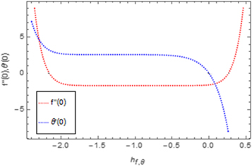
Figure 2. The combined  -curve of
  and
and 
Download figure:
Standard image High-resolution imageTable 1. The convergence table of HAM up to 25th order approximations when Sc = 0.5, Nt = λ = St = M = 0.1, h = −0.5, Pr = Nb = 1.
| Order of approximation | f''(0) | θ'(0)n = 0 |
|---|---|---|
| 1 |

|

|
| 5 |

|

|
| 10 |

|

|
| 15 |

|

|
| 20 |

|

|
| 23 |

|

|
| 25 |

|

|
6. Results and discussion
In this segment we deliberate the physical assets of dissimilar embedding parameters of the modelled problems and there influence on velocity and temperature profile which are showed in figures (3–15). Graphical view of problem is presented in figure 1.

Figure 3. Effect of S on  for dissimilar values, when
Download figure:
Standard image High-resolution image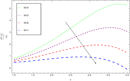
Figure 4. Effect of M on  for dissimilar values, when
Download figure:
Standard image High-resolution image
Figure 5. Effect of K1 on  for dissimilar values,
Download figure:
Standard image High-resolution image
Figure 6. Effect of F1 on  for dissimilar values, when
Download figure:
Standard image High-resolution image
Figure 7. Effect of ε1 on  for dissimilar values, when
Download figure:
Standard image High-resolution image
Figure 8. Effect of M on  for dissimilar values, when
Download figure:
Standard image High-resolution image
Figure 9. Effect of K1 on  for dissimilar values, when
Download figure:
Standard image High-resolution image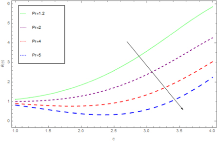
Figure 10. Effect of Pr on  for dissimilar values, when
Download figure:
Standard image High-resolution image
Figure 11. Effect of Ec on  for dissimilar values, when
Download figure:
Standard image High-resolution image
Figure 12. Effect of F1 on  for dissimilar values, when
Download figure:
Standard image High-resolution image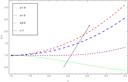
Figure 13. Effect of S on  for dissimilar values, when
Download figure:
Standard image High-resolution image
Figure 14. Effect of ε2 on  for dissimilar values, when
Download figure:
Standard image High-resolution image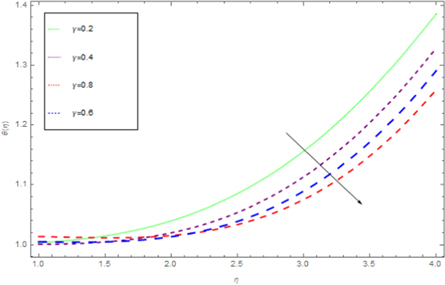
Figure 15. Effect of γ on  for dissimilar values, when
Download figure:
Standard image High-resolution image6.1. Velocity profile 

The present work concentrates on the explanation of the nanoliquid film flow through modelled parameters. Mostly, numerical computations are accomplished for temperature and velocity field distribution contained by the boundary layer film collected with wall velocity and wall temperature gradient, to obtain vision in flow regime of the physics involved of flow parameters for numerous values, which illustrate the structure of flow. Figures 3 to 7 represents the performance of liquid velocity  in the influence of S, inertial parameter F1, magnetic field parameter M, and permeability parameters K1 and ε1 explicitly. We noticed in figure 3 that an increase in the value of S leads to decrease the thickness of film, instantaneously, the inside velocity of thin film increases the surface velocity on raising S. As a result an increase in S increases the stretching velocity
  While slip velocity increases due to raise in slip parameter, and is clearly results in decrease of liquid velocity. We examined in figure 4 that inside thin film liquid, velocity is increased as M increases as well as to reduce radically the film thickness. The reason at the back of such influence of M is due to the introduction of weak body force which is represented as Lorentz force, thin film is an electrically conducting fluid due to the presence of M. This force acts to both the fields in a vertical direction. As viscous force and body force is the ratio of hydro magnetic as suggested by M, higher values of magnetic field shows a greater body force which has the capability to slow down the liquid flow. Figure 5 represent the effect of enlarging of K1, which causes in the reduction the fluid velocity. Since we observed from the appearance of an increase in the value of K1, a reduction in the porous medium permeability. Therefore, small gap is obtainable for fluid to flow and therefore, we examine that velocity of thin film is reduced. Figure 6 illustrates that on rising F1, inner thin film fluid velocity is decreased, while there is no influence of F1 on thickness of film. There is hardly an influence of F1 on free surface velocity which is obvious from figure 6. In state of porous gap with larger pores sizes, and porous medium expended by fluid-solid interaction, which increases the viscous interference. Hence, an increase in F1 causes a better flow resistance, so velocity of fluid is reduces. Figure 7 identifies that ε1 has no influence on fluid film thickness, the reduction of ε1 reduces the fluid velocity.
6.2. Temperature profile θ(η)
Figures 8 to15 are planned to observe the behaviour of θ against the parameters M, K1, Pr, Ec, F1, S, and γ respectively. It is examined from figures 8 to 9 that for larger values of M and K1, temperature of thin film is increased all over in the region of film. While the attainment of permeability parameter and M has led to decrement in the fluid velocity in region of thin film. Thus, additional work is done to slow the fluid against these three physical objects dissipates in the form of energy and therefore enlarged θ is examined in the thermal boundary layer. It is obvious from figure 10 that larger Prandtl number Pr compels to decrease the thin film region the fluid temperature. Increasing Pr, decreases the thickness of thermal boundary layer. Since Pr is a measure of relative significance of thermal diffusivities and momentum, and hence larger the Prandtl number lesser the thermal diffusion. Therefore the results of physical meaning of Prandtl number are in great conformity. Figure 11 identifies that the θ attainment is enlarged on increasing the Ec, which actually supports the physics. Because the ratio of kinetic energy to enthalpy is called Eckert number, heat stored in the liquid is dissipated by increasing Ec, by which the θ is increased. Figure 12 show that an increase F1 means a greater resistance to the flow, therefore, the fluid velocity is getting decreased. Figure 13 shows that fluid temperature is dependent on S. One can examine that when unsteadiness in the stretching increases, which as a result decreases the fluid temperature of thin film as well as free surface temperature. Increasing the values of S a thickened thermal boundary layer is produced. It is exciting to observe at this time that for larger values of S, results in the fluid temperature to fall radically, while the thermal boundary layer get thicker with raise in it. Figure 14 demonstrates that the fluid velocity is decreased on decreasing ε2. Figure 15 shows the effect of γ, which is the similarity variable at free surface given by equation (18), and depends on α. So, in this way that an enlargement in α results in the increment in the value of γ. The values of α is increases due to increase in S and decreases on the increasing values of Eckert number. Therefore, the increasing values of S increases the thickness of the thermal boundary layer. The residual error concentration for velocity and heat profiles are shown in figures (16) and (17) respectively.
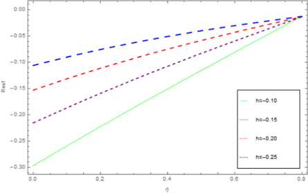
Figure 16. Impact of h curve of the residuals for the velocity.
Download figure:
Standard image High-resolution image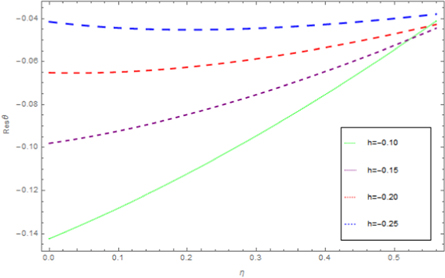
Figure 17. Impact of h curve of the residuals for the temperature.
Download figure:
Standard image High-resolution image
6.3. Table discusssion
Tables 2–4 describes the impact of Cfx and Nu under the effect of different parameters. The properties of M, Ec, ε2 and s on skin friction for the different values are shown in table 2. It is examined that the increasing rates of magnetic M and unsteady parameter S blows the Skin-friction coefficient. The higher values of stretching parameter ξ and thickness constraint β reduces the Cfx coefficient. The effects of M, s, Ec and Pr on the Nu for the different values are shown in table 3. It is observed that increasing rates of unsteady parameter S and magnetic parameter M reduces the Nu, while the unsteady parameter s, and β increase the Nu. The effects of M, Rd, Pr and s on the Nu is shown in table 4. It is noticed that Nu increases due to an increase in thermoporetic parameter, while increasing unsteady parameter and Pr causes a decreases Nu.
Table 2. The Skin friction coefficient for different values of M, k, ε1 and S.
| M | k | ε1 | S | Cfx |
|---|---|---|---|---|
| 0.1 | 0.5 | 0.1 | 1.5 |

|
| 0.5 |

|
|||
| 1.0 |

|
|||
| 1.5 | 0.1 |

|
||
| 0.5 |

|
|||
| 1.0 |

|
|||
| 1.5 | 0.1 |

|
||
| 0.5 |

|
|||
| 1.0 |

|
|||
| 1.5 | 0.1 |

|
||
| 0.5 |

|
|||
| 1.0 |

|
Table 3. When Pr = 6 or 7 variation in Nusselt number for different values of M, ε2, S, Ec and γ.
| M | ε2 | S | Ec | γ | Nux |
|---|---|---|---|---|---|
| 0.1 | 0.1 | 1.5 | 1.5 | 0.1 |

|
| 0.5 |

|
||||
| 1.0 |

|
||||
| 1.5 | 0.1 |

|
|||
| 0.5 |

|
||||
| 1.0 |

|
||||
| 1.5 | 0.1 |

|
|||
| 0.5 |

|
||||
| 1.0 |

|
||||
| 1.5 | 1.5 |

|
|||
| 3.0 | 0.5 |

|
|||
| 5.0 | 2.0 |

|
|||
| 7.0 | 3.0 |

|
Table 4. Variation in Nusselt umber for different values of M, Pr, Rd and St.
| Present result | Previous results [44] | |||
|---|---|---|---|---|
| S | γ |

|
γ |

|
| 0.4 | 4.981 455 | −1.134 098 | 4.981 004 | −1.134 09 |
| 0.6 | 3.131 710 | −1.195 128 | 3.131 710 | −1.195 10 |
| 0.8 | 2.151 990 | −1.245 805 | 2.151 990 | −1.245 76 |
| 1.0 | 1.543 617 | −1.277 769 | 1.543 600 | −1.277 66 |
| 1.2 | 1.127 780 | −1.279 171 | 1.127 800 | −1.278 85 |
| 1.4 | 0.821 033 | −1.233 545 | 0.821 032 | −1.233 49 |
| 1.6 | 0.576 176 | −1.114 941 | 0.576 170 | −1.114 83 |
| 1.8 | 0.356 390 | −0.867 416 | 0.356 389 | −0.867 42 |
7. Conclusion
Concerning to frequent uses in the engineering field and the study of industrial devices, we have presented a mathematical model for defining the fluid film flow of non-Newtonian nano-fluids through malleable viscidness and thermal conductivity in occurrence of uniform magnetic field. The model of the flow is invented for nano-liquids over a stretching sheet. We are strongly trusted in this modification efforts to be worthy enough for the investigators to classify the unlimited thermal conductive, non-Newtonian fluid with unlimited thermal conductive nanoparticles. The key determined comments of this work are:
- It is investigated that for large values of M that the nanofluid films velocity distribution decreases.
- Thickness of thermal boundary layer decreases with increasing values of S, while increase of radiation parameter, the Nusselt number also increases.
- It is observed that increase in the value of K1, a reduction in the porous medium permeability.
- The increasing values of Pr, increases the surface temperature, where inverse influence is create for S, that the surface temperature reduces due to large values of S.
- An increase temperature profile is observed for greater values of Eckert number Ec and vice versa.
- The mass flux decreases due to greater values of S, while a decrease in S causes an increase in the mass flux.
- HAM method convergence with the variations in physical parameters is examined numerically.
Competing interests
All the authors declare that they have no challenging interests.