
Abstract
The purpose of the study is to investigate the dynamic mechanical properties and constitutive relationship of martensitic stainless steel 0Cr17Ni4Cu4Nb. For this purpose, the impact test was performed at six strain rates (750, 1500, 2000, 2600, 3500, and 4500 s−1) and four temperatures (25, 350, 500, and 650 °C) by using the high-temperature split Hopkinson pressure bar (SHPB) test device to attain the stress–strain relationship of materials; in addition, quasi-static (0.001, 0.01, and 0.1 s−1) compression tests were conducted by applying the UTM5305 universal testing machine at normal temperature. The analysis of the stress–strain curves indicates that the stainless-steel shows strain-rate strengthening and thermal softening and the adiabatic temperature rise during the plastic deformation at a high strain rate exerts a thermal softening effect on materials. With the aid of Johnson-Cook (J-C) and power-law (P-L) constitutive models, the dynamic constitutive relation of the martensitic stainless steel 0Cr17Ni4Cu4Nb was fitted and the correlation coefficients (R) and average absolute relative errors (AAREs) obtained through use of the two constitutive models were compared. Results indicate that the curves obtained through the constitutive models match the test curves to a reasonable extent. The R values are 0.968 33 and 0.977 80 while AAREs obtained through the J-C and P-L models are 4.77% and 2.25%, respectively. It can be found that the P-L model is slightly superior to the J-C model in terms of fitting accuracy. In addition, the dynamic mechanical properties of the materials were assessed through use of their constitutive equations from the perspectives of strain-rate sensitivity and temperature sensitivity and the acquired results are relatively consistent with the test results.
Export citation and abstract BibTeX RIS

Original content from this work may be used under the terms of the Creative Commons Attribution 4.0 licence. Any further distribution of this work must maintain attribution to the author(s) and the title of the work, journal citation and DOI.
1. Introduction
0Cr17Ni4Cu4Nb, as a typical martensitic precipitation hardening stainless steel, is widely applied in aerospace (turbine blades), nuclear power (steam turbine blades), and chemical engineering machinery (offshore platforms) by virtue of its favorable corrosion resistance, heat resistance, and mechanical properties [1–4]. Therein, the material works in a complex environment and is difficult to machine using dynamic load in the working and machining processes, therefore, it is necessary to explore the dynamic mechanical properties of 0Cr17Ni4Cu4Nb stainless steel.
A constitutive equation, showing the relationships of the flow stress of materials with the strain, temperature, and strain rate, reflects the dynamic response of materials to thermodynamic parameters during dynamic loading and provides an important basis for finite element software as used to perform numerical simulation of the plastic deformation of materials [5–7]. At present, the widely used constitutive models include Johnson-Cook (J-C), Zerilli-Armstrong (Z-A), power-law (P-L), and Arrhenius models [8, 9], in which J-C and P-L models, as two classical constitutive models, can reflect the strain-induced strengthening, strain-rate strengthening, and thermal softening effects [10, 11]. In recent years, scholars have investigated the mechanical properties of, and constitutive models used for stainless steel, which provides a basis for the present study. Z He et al [1] explored the dynamic stress–strain relationships of 0Cr17Ni4Cu4Nb stainless steel at multiple strain rates to construct the Cowper-Symonds (C-S) dynamic strengthening model and analyze the similarities and disparities between the engineering stress–strain and true stress–strain of materials. L Wu et al [11] assessed the dynamic mechanical behavior of stainless steel FV520B and fitted J-C and P-L models thereto. The results predicted through use of the J-C and P-L models match the experimental results, in which the P-L model delivers the higher prediction accuracy. B Shang et al [12] surveyed the quasi-static stress–strain relationships of 0CrlTMn5Ni4M03Al stainless steel at different temperatures (25, 300, and 500 °C) and at the same strain rate (0.0005 s−1) and the dynamic mechanical properties at different temperatures (25, 300, 500, and 700 °C) and different strain rates (300, 1000, and 2700 s−1); moreover, a modified J-C constitutive model was established. The test results indicated that the stainless-steel exhibits strain-rate strengthening and thermal softening and the results predicted by the modified J-C constitutive model are favorably coincident with experimental results. Y L Wang et al [13] explored the dynamic mechanical properties of the high-nitrogen austenitic stainless steel at different temperatures (200 ∼ 600 °C) and different strain rates (100 ∼ 1,000 s−1) and established the J-C constitutive model. The test results show that the materials exhibit both strain and temperature sensitivities and the results obtained through the J-C constitutive model are consistent with the test results. By simulating thermal compression test regimes, X N Cheng et al [14] investigated the deformation behaviors of 316 L austenitic stainless steel at different temperatures (900 ∼ 1100 °C) and low strain rates (0.01 ∼ 5 s−1). Based on the Arrhenius model, the modified constitutive equation was established with consideration of strain duly included. The results implied that the flow stress on 316L stainless steel is high at a low temperature and a large strain rate; the correlation coefficient (R) and average absolute relative error (AARE) between the predicted value and test value are 0.986 88 and only 4.6%, respectively, which indicates that the model can predict the deformation resistance. At present, the dynamic mechanical properties and J-C and P-L constitutive models for martensitic stainless steel 0Cr17Ni4Cu4Nb were rarely investigated, therefore, the dynamic mechanical properties and J-C and P-L constitutive models for martensitic stainless steel 0Cr17Ni4Cu4Nb were explored with the aid of the quasi-static testing machine and a machine designed to measure various dynamic mechanical properties.
By using the UTM5305 universal testing machine and utilizing the high-temperature split Hopkinson pressure bar (SHPB) test device (ALT1000), quasi-static (0.001, 0.01, and 0.1 s−1 at room temperature) compression tests and dynamic impact tests (at temperatures of 25, 350, 500, and 650 °C and strain rates of 750, 1500, 2000, 2600, 3500, and 4500 s−1) were separately performed. On this basis, the true stress–strain curves were attained and the dynamic mechanical properties of martensitic stainless steel 0Cr17Ni4Cu4Nb were analyzed. Additionally, the J-C and P-L constitutive models were used as predictive tools; the accuracies of the two models were compared according to R and AARE, offering a basis for choice of parameters in future numerical simulation.
2. Tests
The materials used were 0Cr17Ni4Cu4Nb bars with the diameter of 30 mm produced by Shanghai Baosteel Group Corporation, China and their chemical composition is displayed in table 1.
Table 1. Chemical composition of 0Cr17Ni4Cu4Nb stainless steel (mass fraction/ %).
| Element | C | Si | Cr | Ni | Mn | P | S | Cu | Nb | Fe |
|---|---|---|---|---|---|---|---|---|---|---|
| Ingredient | 0.06 | 0.80 | 16.25 | 3.60 | 0.82 | 0.03 | 0.02 | 3.83 | 0.28 | Bal. |
Before the test, the materials were first processed into cylindrical specimens with dimensions of Φ3 mm × 3 mm through wire cutting after undergoing solid solution treatment (heating to 1040 °C, holding for 10 ∼ 15 min, and then air-cooling). The verticality of the end faces to the cylindrical surface was guaranteed; afterwards, the two end faces of specimens were polished with silicon carbide finishing paper to ensure the surface roughness Ra was no greater than 1.6 μm. The UTM5305 universal testing machine and the ALT1000 high-temperature SHPB test device used in the present research are shown in figures 1 and 2, respectively. During high-temperature testing, the specimens were heated using the synchronously assembled heating system; the high-temperature heating furnace and temperature control system are illustrated in figure 3. Thermocouple wires were used to fix specimens to the casing and the casing could slide along the incident bar at will. When heating the specimen, the incident bar and transmission bar were kept away from the heating furnace, and the temperature in the furnace was maintained at a preset value by virtue of the temperature control system. After reaching the preset temperature, the specimen was held for more than 5 min to guarantee uniform heating. During testing, the lengths of the impact rods for the test and the diameter of the pressure bars were 100 mm and 8 mm, respectively. To reduce error in the test, the shaping technology of stress waves was applied, and a rubber sheet was added to the loaded end of the incident bar as a shaer, resulting in smooth signals from both the incident and reflected waves. This guaranteed consistency between strain at the measuring point and actual strain at the loading point. In addition, the test was conducted three times under each condition and then the test values were averaged to ascertain the stress–strain relationship figure 4 shows the macro-morphologies of the specimen before and after (quasi-static) compression and (dynamic) impact at 25 °C.

Figure 1. UTM5305 universal testing machine.
Download figure:
Standard image High-resolution image
Figure 2. SHP impact device.
Download figure:
Standard image High-resolution image
Figure 3. Heating system.
Download figure:
Standard image High-resolution image
Figure 4. Macro-morphology before and after compression (quasi-static) and impact (dynamic) at different strain rates at 25 °C.
Download figure:
Standard image High-resolution image3. Test results and analysis
3.1. Analysis of the stress–strain relationship
Under quasi-static conditions, the stress–strain curves under load at different strain rates (0.001, 0.01, and 0.1 s−1) are shown in figure 5. Under dynamic conditions, the stress–strain curves loaded at the same temperature (25 °C) and different strain rates (750, 1500, 2000, 2600, 3500, and 4500 s−1) are illustrated in figure 6. As shown in figures 5 and 6, the dynamic stress–strain curve in the initial stage at a high strain rate presents an increasing slope and enters a plastic stage thereafter. In this case, the materials are subject to plastic deformation. Due to the generation of a dislocation, the stress increases slowly with the strain (albeit to an insignificant extent), indicating that the materials have entered a stage of steady plastic deformation.

Figure 5. The true stress-strain curve of 0Cr17Ni4Cu4Nb stainless steel under quasi-static conditions.
Download figure:
Standard image High-resolution image
Figure 6. The true stress-strain curve of 0Cr17Ni4Cu4Nb stainless steel at room temperature.
Download figure:
Standard image High-resolution image3.2. Analysis of strain-rate sensitivity
It can be seen from figure 6 that the materials show a certain strain-rate strengthening effect. To quantify the influence of the strain rate on the stress on such materials, a strain-rate sensitivity parameter β is introduced, which is defined as follows [15, 16]:

where,  and
and  separately refer to the measured stresses in the quasi-static state (
 ) and high strain rates (
 = 2600, 3500, or 4,500 s−1).
The strain-rate sensitivity is calculated based on the test data, as shown in table 2: the strain-rate sensitivity of the materials increases with the growing strain rate while decreases with increasing strain, showing the strain-rate strengthening effect.
Table 2. Strain rate sensitivity parameters of 0Cr17Ni4Cu4Nb stainless steel.
Strain Rate 
| True strain 
| Strain rate sensitivity 
|
|---|---|---|
| 2600 | 0.08 | 56.8 |
| 0.10 | 44.0 | |
| 0.12 | 36.7 | |
| 0.14 | 32.2 | |
| 3500 | 0.08 | 61.4 |
| 0.10 | 50.7 | |
| 0.12 | 43.4 | |
| 0.14 | 39.6 | |
| 4500 | 0.08 | 62.3 |
| 0.10 | 51.0 | |
| 0.12 | 44.0 | |
| 0.14 | 42.1 |
3.3. Analysis of the temperature sensitivity
The stress–strain curve of the 0Cr17Ni4Cu4Nb stainless steel at a strain rate of 4500 s−1 and different temperatures is shown in figure 7: the materials deliver the temperature sensitivity, that is, the stress decreases with increasing temperature. To assess the influence of temperature on the stress on a material, the temperature sensitivity nt is introduced, which is defined as follows [15, 16]:

where,  and
and  represent the corresponding stresses under a certain strain at the same strain rate and test temperatures of
  and
and  respectively.

Figure 7. The true stress-strain curve of 0Cr17Ni4Cu4Nb stainless steel at different temperatures ( ).
).
Download figure:
Standard image High-resolution imageThe temperature sensitivity is calculated according to the test data (table 3): the temperature sensitivity of the materials increases with the temperature, evincing the thermal softening effect. The effect is caused by the synergistic effect of the test temperature and an adiabatic temperature rise at a high strain rate. The adiabatic temperature rise during material deformation at a high strain rate is generally calculated according to the following equation [17–20]:

where, 

 and
and  denote the true stress, true strain, material density, and specific heat capacity of materials, respectively;
  represents the work to heat conversion factor and
  = 0.9 [21, 22]. As for the specimens,
  and
and 
Table 3. Temperature sensitivity parameters of 0Cr17Ni4Cu4Nb stainless steel ( ).
).
Temperature range 
| True strain 
| Temperature sensitivity 
|
|---|---|---|
| 25–350 | 0.06 | 0.032 |
| 0.10 | 0.029 | |
| 0.14 | 0.039 | |
| 0.18 | 0.043 | |
| 25–500 | 0.06 | 0.047 |
| 0.10 | 0.049 | |
| 0.14 | 0.053 | |
| 0.18 | 0.058 | |
| 25–650 | 0.06 | 0.081 |
| 0.10 | 0.078 | |
| 0.14 | 0.083 | |
| 0.18 | 0.083 |
Based on the data in figure 7, the adiabatic temperature rise is calculated according to equation (3). Figure 8 displays the adiabatic temperature rise of materials at a strain rate of 4500 s−1 and different temperatures. It can be seen from the figure that an increase of strain corresponds to the growth of the adiabatic temperature rise of materials, which is attributed to the accumulation of heat generated during the plastic deformation of the materials. The adiabatic temperature rise of materials decreases with increasing test temperature. The increase in temperature generally causes material softening. At a high strain rate, the strain hardening of materials competes with that induced by adiabatic temperature.

Figure 8. Adiabatic temperature rise under different temperatures ( ).
).
Download figure:
Standard image High-resolution image4. Establishment of the constitutive models
4.1. J-C constitutive model
The J-C model [23–27] can reflect the work hardening effect, strain-rate effect, and thermal softening effect of materials, which is expressed as follows:


where, 


 and
and  refer to the yield stress on materials, the yield strength at the reference temperature and reference strain rate (quasi-static state), strain hardening coefficient, strain hardening index, strain-rate hardening coefficient, and thermal softening index, respectively; the equivalent plastic strain is given by
  where
where  and
and  separately denote the plastic strain and reference strain;
  denotes the dimensionless plastic strain rate, where
  and
and  refer to the reference strain rate and plastic strain rate;

 and
and  denote the relative temperature, reference temperature, the melting point of the material, and the instantaneous temperature, respectively.
At first, the first term in the right side of the J-C constitutive equation corresponds to the normal temperature and strain rate. The J-C constitutive model is expressed as follows:

The constants in the machining process of materials are determined according to the quasi-static compression test of the material at normal temperature. As shown in figure 5 (corresponding to a strain rate of 0.01 s−1), the yield strength of the materials is 1050.95 MPa ( ) and the reference strain is 0.01. Through transposition according to equation (6), it can be found that:

By taking the logarithm of both sides of equation (7), it can be found that:

Therefore, the slope  (
( ) of the curve and
  are attained through fitting (figure 9).

Figure 9. The first fitting curve of the Johnson-Cook model.
Download figure:
Standard image High-resolution imageAccording to the equation,

It is found that:

By taking the reference strain rate as 100 s−1, linear fitting is applied to obtain  as illustrated in figure 10.

Figure 10. The second fitting curve of the Johnson-Cook model.
Download figure:
Standard image High-resolution imageAccording to the equation,

By taking the logarithm of both sides of equation (11), it can be found that:

Finally, the value of the thermal softening term  of materials is determined according to the experimental stress–strain curve at a high strain rate (4500 s−1) and different temperatures (the melting point of the material is taken as
  ). On this basis, linear fitting (figure 11) gives
  The parameters of the J-C model are summarized in table 4.
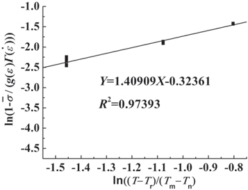
Figure 11. The third fitting curve of the Johnson-Cook model.
Download figure:
Standard image High-resolution imageTable 4. Parameters for the Johnson-Cook model.
| A/MPa | B/MPa | n | C | m |
|---|---|---|---|---|
| 1050.95 | 17.677 | 0.5302 | 0.1018 | 1.409 09 |
Eventually, the J-C constitutive equation for martensitic stainless steel 0Cr17Ni4Cu4Nb at a high strain rate is expressed as follows:

4.2. P-L constitutive model
The P-L model [28–30] can also reflect the work-hardening, strain-rate effect, and thermal softening of materials, which is expressed as follows:


where, 


 and
and  denote the strain hardening index, strain-rate strengthening index, the initial test temperature, adiabatic temperature rise, yield strength at the reference temperature and reference strain rate, plastic strain, reference strain, plastic strain rate, and reference strain rate, respectively; C0, C1, ... and C5, separately represent the polynomial coefficients of temperature.
At first,  and
and  of materials are deduced. By using the experimental stress–strain relationship of materials in a quasi-static state (that at a strain rate of 0.01 s−1) and supposing that both the strain-rate strengthening term
  and thermal softening term
  are equal to 1, equation (14) is simplified as follows:

By separately fitting the straight lines in the elastic and plastic stages of the experimental stress–strain curve, the point of intersection of two straight lines corresponds to the yield strength, that is,  moreover, equation (19) is solved by taking the reference strain as 0.001 and the logarithms of both sides of the equation are simultaneously calculated, giving:

The slope ( ) of the straight line is determined as 0.038 52 by substituting the corresponding true stress of the strain within 0.25 ∼ 0.41 and corresponding strains into equation (20) and then the linear fitting is performed. Furthermore,
  is obtained, as shown in figure 12.

Figure 12. Relationship between  and
and 
Download figure:
Standard image High-resolution imageThe value of  materials is determined according to the true stress–strain curve at normal temperature and strain rates between 750 ∼ 4500 s−1. It is supposed that the thermal softening term
  is equal to 1 and thus equation (14) can be simplified as follows:

By taking the logarithms of both sides of equation (21), it can be found that:

By setting the reference strain rate as 1900 s−1 and substituting the measured stress at strains of 0.05 and 0.06 and corresponding strain rates into equation (22), linear fitting is conducted. On this basis, the slope  of the straight line is determined as 0.166 35 and furthermore
  as illustrated in figure 13.

Figure 13. Relationship between  and
and 
Download figure:
Standard image High-resolution imageThe temperature terms C0, C1, ... and C5 are determined according to the experimental stress–strain curves at temperatures between 25 °C ∼ 650 °C and strain rates of 750 ∼ 4500 s−1. Equation (14) is transformed as follows:

Considering the influence of adiabatic temperature rise ( ) on the plastic deformation of materials, by substituting the actual stresses at different temperatures into equation (23) and performing polynomial fitting, it can be found that C0 = 0.976 14, C1 = 1.424 45 × 10−5, and C2 = −5.1262 × 10⁻⁷. The fitting curves are shown in figure 14. The parameters of the P-L model are summarized in table 5.
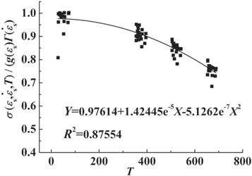
Figure 14. Relationship between  and
and 
Download figure:
Standard image High-resolution imageTable 5. Parameters for the power-law model.
| σ0/MPa | 1/n | 1/m | C0 | C1 | C2 |
|---|---|---|---|---|---|
| 1050.95 | 0.038 52 | 0.166 35 | 0.976 14 | 1.424 45 × 10−5 | −5.1262 × 10⁻⁷ |
Finally, the P-L constitutive equation for martensitic stainless steel 0Cr17Ni4Cu4Nb at a high strain rate is shown as follows:

Figure 15 compares the values of true stress predicted by the J-C and P-L constitutive models with the test values under different conditions. The further to investigate the accuracies of the two models, the error analysis is performed by using the mean absolute error (MAE) (Δσ), R and AARE, which are expressed as follows [31–36]:


where,  and
and  separately refer to the test and predicted values of the true stress (MPa);
  and
and  separately denote the means of
  and
and 
 represents the total number of data points used here. The MAEs are summarized in table 6 and R values and AAREs are displayed in figure 16.

Figure 15. Power-law and Johnson-Cook constitutive model predictions and measured values.
Download figure:
Standard image High-resolution imageTable 6. Absolute error mean value in the two constitutive models under different deformation conditions.

|

|

|

|
|---|---|---|---|
| 25 | 750 | 27.62 | 28.26 |
| 1500 | 24.15 | 50.54 | |
| 2000 | 23.37 | 48.60 | |
| 2600 | 15.45 | 74.33 | |
| 3500 | 34.94 | 22.39 | |
| 4500 | 22.55 | 19.79 | |
| 350 | 750 | 32.24 | 7.89 |
| 1500 | 17.07 | 16.85 | |
| 2000 | 26.69 | 46.84 | |
| 2600 | 47.22 | 16.36 | |
| 3500 | 17.90 | 57.23 | |
| 4500 | 36.01 | 32.49 | |
| 500 | 750 | 58.22 | 19.79 |
| 1500 | 24.63 | 57.20 | |
| 2000 | 20.66 | 74.87 | |
| 2600 | 32.57 | 54.25 | |
| 3500 | 17.86 | 89.96 | |
| 4500 | 35.37 | 82.03 | |
| 650 | 750 | 17.88 | 86.16 |
| 1500 | 10.65 | 96.21 | |
| 2000 | 27.81 | 102.54 | |
| 2600 | 50.67 | 59.97 | |
| 3500 | 18.84 | 107.39 | |
| 4500 | 19.93 | 120.29 |

Figure 16. The correlation between the true stress prediction and experimental values from power-law and Johnson-Cook constitutive models.
Download figure:
Standard image High-resolution imageAccording to figure 15 and table 6, it can be found that the values predicted by the J-C and P-L models differ from the test values under the same deformation conditions. Under most deformation conditions, the MAE of the P-L model is smaller than that of the J-C model. The maximum MAE (58.22 MPa) of the P-L model is determined at 500 °C and 750 s−1 while that (120.29 MPa) of the J-C model occurs at 650 °C and 4500 s−1. Overall, as the temperature rises, the MAE of the P-L model varies to an insignificant extent and is stable while that of the J-C model gradually increases, which reaches a maximum at 650 °C. This is ascribed to the difference of the third terms in expressions of the two models. The third term in the P-L model is expressed by using a polynomial while that in the J-C model is shown as the relative exponent. The P-L model is slightly superior to the J-C model and it shows higher accuracy at high temperature.
Figure 16 compares the correlations of the values of the true stress predicted by the two models with the test values: the R values are 0.977 80 and 0.968 33 while AAREs of the P-L and J-C models are 2.25% and 4.77%, respectively. The P-L model is shown to deliver higher prediction accuracy than the J-C model and it can better predict the stress on martensitic stainless steel 0Cr17Ni4Cu4Nb.
5. Dynamic mechanical properties based on the P-L constitutive model for stainless steel 0Cr17Ni4Cu4Nb
5.1. Strain-induced strengthening effect
In the case that the strain rate and temperature are kept constant, the derivative of the strain at 25 °C and 750 s−1 is found from equation (24), as shown in figure 17. In the figure, the derivative is greater than 0, indicating that the stress increases with the strain (i.e. the strain-induced strengthening effect); however, when the strain reaches a certain value, the derivative tends to 0. This implies that the growth in stress gradually decreases and the stress gradually stabilizes, which is in agreement with the experimental results.

Figure 17. Sensitivity to strain strengthening.
Download figure:
Standard image High-resolution image5.2. Strain-rate strengthening effect
The derivative of the strain rate under the strain of  is obtained using equation (24) when the strain and temperature are constants, as shown in figure 18, in which the derivative is greater than 0, which indicates that the actual stress increases with increasing strain rate (i.e. the strain-rate strengthening effect); however, the derivative drops as the strain rate is further increased, suggesting that the strain-rate strengthening effect is gradually weakened, being consistent with the experimental results.

Figure 18. Sensitivity to strain-rate strengthening ( ).
).
Download figure:
Standard image High-resolution image5.3. Thermal softening effect
On condition that the strain and strain rate are kept constant, the temperature at a strain of  is calculated by using equation (24), as shown in figure 19. It can be seen from the figure that the derivative is less than 0, implying a reduction in stress with increasing temperature (i.e. the thermal softening effect); this matches the experimental results.

Figure 19. Sensitivity to temperature softening ( ).
).
Download figure:
Standard image High-resolution image
6. Conclusion
Taking martensitic stainless steel 0Cr17Ni4Cu4Nb as the research object, quasi-static and dynamic impact tests were conducted on the universal testing machine and the high-temperature SHPB test device, and the following conclusions were drawn:
- (1)The martensitic stainless steel 0Cr17Ni4Cu4Nb exhibits strain-rate strengthening and thermal softening effects.
- (2)The J-C and P-L constitutive models can predict the behavior of martensitic stainless steel 0Cr17Ni4Cu4Nb. Based on the P-L and J-C models, the R values are 0.977 80 and 0.968 33 while AAREs between the predicted values and test values are 2.25% and 4.77%, respectively. By contrast, the fitting accuracy of the P-L model is slightly better than that of the J-C model.
- (3)The two constitutive models both have certain errors that change in different ways with increasing strain rate and temperature. This is mainly because the stress–strain curve under high-temperature, high-stress conditions is highly non-linear and the coupling of the strain, strain rate, and temperature is not considered when determining parameters of the constitutive models.
- (4)The dynamic mechanical properties of the materials were investigated according to the constitutive equations from the perspectives of strain-rate sensitivity and temperature sensitivity, which are consistent with the test results.
Acknowledgments
This work was financially supported by the National Natural Science Foundation of China (No. 51965031and No. 51865026), Gansu Youth Science and Technology Fund Project (No. 21JR7RA351), Gansu Province Higher Education Innovation Fund Project (No. 2019B-179, 2021A-156 and 2021B-319), Lanzhou Institute of Technology 'Qizhi' Talent Training Program (No.2018QZ-03).
Data availability statement
All data that support the findings of this study are included within the article (and any supplementary files).