DIFFUSION OF SOLAR MAGNETIC ELEMENTS UP TO SUPERGRANULAR SPATIAL AND TEMPORAL SCALES

F. Giannattasio; D. Del Moro; F. Berrilli; L. Bellot Rubio; M. Gos˘ić; D. Orozco Suárez

doi:10.1088/2041-8205/770/2/L36

1. INTRODUCTION

The interaction of magnetic fields with the convective plasma flows of the solar photosphere significantly affects the Sun's activity. In solar magnetohydrodynamics (MHD) theories of coronal heating, such an interaction is invoked in various ways (see, e.g., Alfvén 1947; Parker 1988; Hughes et al. 2003; Viticchié et al. 2006; Dikpati & Gilman 2006; De Pontieu et al. 2007; Tomczyk et al. 2007; van Ballegooijen et al. 2011; Stangalini et al. 2011, 2012; Harra & Abramenko 2012).

Photospheric flows concentrate and advect the magnetic field, and eventually organize it, on different spatial and temporal scales. In a few minutes, the magnetic field is advected from the interior of the granules to the intergranular lanes (e.g., Del Moro 2004; Centeno et al. 2007). The field is organized on mesogranular scales on timescales of hours (e.g., November 1980; Roudier et al. 1998; Berrilli et al. 2005b; Yelles Chaouche et al. 2011; Berrilli et al. 2013) and is transported to the supergranular boundaries on timescales of days (e.g., Hart 1956; Simon & Leighton 1964; Berrilli et al. 2004; De Rosa & Toomre 2004; Del Moro et al. 2004, 2007; de Wijn et al. 2008; Orozco Suárez et al. 2012).

Under the hypothesis that the magnetic field is passively transported by the velocity field, the motion of magnetic concentrations is a manifestation of the underlying organizing processes and may be described in terms of a diffusion process. Such a hypothesis requires that the drag force F_d due to the plasma kinetic energy be much greater than the magnetic force F_b exerted by the magnetic elements on the surroundings, i.e., F_d ≫ F_b (Petrovay 1994).

The diffusion process can be represented by the law 〈(Δl)²〉 ∼ τ^γ (see, e.g., Cadavid et al. 1999), which describes the way the mean-squared displacement of magnetic concentrations 〈(Δl)²〉 grows with time τ. When the spectral index γ is unity, the process involved is called normal diffusion, and the above equation reads 〈(Δl)²〉 = 4Kτ, where K is the diffusion coefficient. The case γ ≠ 1 is referred to as anomalous diffusion. In this case the quantity K(τ) = 〈(Δl)²〉/4τ is not a constant and scales as a power law K(τ) = τ^{γ − 1}. When γ > 1, the diffusion coefficient increases with both the spatial and temporal scales (superdiffusion); when γ < 1, the diffusion coefficient decreases when the scale increases (subdiffusion).

Several works investigated the diffusion of magnetic fields on the photosphere, and the results are often conflicting. Most studies rely on magnetic proxies like G-band bright points to track the magnetic field advection (see, e.g., Berger et al. 1998; Cadavid et al. 1998, 1999; Lawrence et al. 2001; Sánchez Almeida et al. 2010; Abramenko et al. 2011). In contrast, the works of Wang (1988), Hagenaar et al. (1999), and Manso Sainz et al. (2011) used magnetograms to describe the diffusion process. Most of those authors agreed in finding a superdiffusive transport regime, but they obtained different diffusion coefficients. Also, they often reported that the diffusion coefficient changes with the spatial and temporal scales. None of those works, however, could take advantage of a data set spanning all of the spatial (from subgranular to supergranular) and temporal (from a few seconds to days) scales involved in the magnetic diffusion process.

Indeed, to probe the smallest and fastest scales, high spatial resolution and high cadence observations are required, while large field of view and long duration data sets are essential to investigate the large spatial and extended timescales present in the solar surface. Moreover, space-borne solar observations are essential to avoid effects introduced by Earth's atmosphere, which limit the spatial resolution and potentially superpose spatial and temporal turbulent scales on the observed magnetic diffusion process. Hinode magnetograms permitted us to explore the diffusion properties of 20,145 magnetic concentrations (magnetic elements) at unprecedented spatial and temporal scales. These measurements, taken under seeing-free conditions combine high spatial resolution (0 farcs 3) in all the fields of view and long duration (∼25 hr without interruption). Moreover, tracking elements using magnetograms instead of magnetic proxies, as G-band bright points, eliminates a possible source of contamination in the selection (de Wijn et al. 2008; Viticchié et al. 2010).

2. OBSERVATIONS AND DATA ANALYSIS

2.1. The Hinode Data Set

Our data set consists of a magnetogram time series of a quiet-Sun region at the disk center. The spectral line used is Na i D 589.6 nm, observed at two wavelengths (±160 mÅ from the line center) with the Hinode Narrowband Filter Imager (NFI; Kosugi et al. 2007; Tsuneta et al. 2008). The data are 2 × 2 binned, corresponding to a pixel area of 0.16 × 0.16 arcsec² and a spatial resolution of 0 farcs 3. The magnetogram noise, computed as the rms fluctuation of the signal in a region without magnetic fields, is σ = 6 Mx cm⁻² (or 6 G) for individual frames, making this the highest sensitivity ever achieved in magnetographic observations of the quiet Sun.

The series starts at 08:00:42 UT on 2010 November 2 and lasts for 25 hr without interruption at a cadence of 90 s (995 frames). The data have been coaligned, trimmed to the same field of view, and filtered for five minute oscillations as explained by Gos˘ić (2012). The large field of view (about 51 × 53 Mm²) allows us to observe a whole supergranular cell as well as surrounding quiet-Sun areas (Figure 1). The magnetogram reported in this figure has been saturated at ±10 G. It does not show individual internetwork elements because they do not stay at the same position for long.

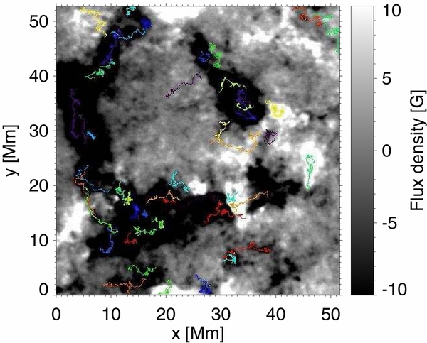
**Figure 1.** Mean magnetogram saturated at ±10 G. The colored tracks represent the trajectories of the 50 longest living magnetic elements. Their lifetimes span the range from ∼4 to ∼11 hr.
Download figure:
Standard image High-resolution image

2.2. Tracking the Magnetic Elements

Since segmenting the magnetograms with a single threshold leads to either the loss of weak magnetic structures or the merging of strong magnetic structures in big clusters (Berrilli et al. 2005a), we implemented an iterative procedure to resolve both the weak B structures and the peaks of the larger magnetic features. The segmented temporal sequence is then used to reconstruct the trajectory of the magnetic features.

The segmentation of each image is obtained as follows: a starting threshold is defined as T₀ = 3σ (three times the noise level) and all the pixels whose |B(x, y)| > T₀ are flagged as magnetic pixels, and the rest is discarded. All the flagged pixels which are clustered in groups smaller than A_max = 50 pixels (corresponding to an equivalent diameter of ≲ 1 arcsec) are recognized as segmented features and labeled. The rest of the flagged pixels (composed of large connected regions) are instead selected for the next iteration with a threshold T₁ raised by ΔT = 3σ. The process is iterated until there are no more connected regions larger than A_max in the image. In the network, this separates the magnetic fluxes into small-scale structures around the local maxima.

The tracking of the segmented features is done as in Del Moro (2004). The labeled structures are tracked forward in time from the first frame of their detection with the following rules. Each structure present in the next frame whose center is within a distance R from the original structure is compared in shape with the original one. The closest match (the maximum allowed discrepancy is 150%) is retained as the evolution of the original element. The distance R is a parameter of the tracking algorithm and has been set to 3 arcsec for this data set. If the search in the next frame fails, it is extended to the two next frames, otherwise it stops and the trajectory of the structure ends. Once all the labeled structures in a frame have been examined, the algorithm processes the next frame. All the features successfully tracked for more than four frames are used in the following analysis. Since the shape difference between features is computed as the percentage of non-overlapping pixels in the feature superposition, the 150% maximum allowed deformation value allows for the rotation of small and elongated features.

According to these criteria, 20,145 magnetic elements were tracked in 25 hr. Their lifetimes range from 7.5 minutes to 11.1 hr. We note that the lower lifetimes are artificial, due to the selection criteria.

3. RESULTS

3.1. The Lifetime of Magnetic Elements

The mean magnetogram shown in Figure 1 allows us to locate the most "persistent" magnetic fields, which settle mainly on the edges of the supergranule (SG). In the same figure, the tracks corresponding to the 50 longest living magnetic elements are represented. We define the network as the region where |B| > 25 G in the mean magnetogram. The polygonal region confined by the network is defined to be the SG (network included).

The location of the last appearance has been used to decide whether each magnetic element belongs to the inner SG, the network, or the rest of the frame. We found that the SG hosts a total of 10,123 magnetic elements, 2522 of which lie on the network. The remaining 10, 022 magnetic elements are outside the SG.

In Figure 2 we show the magnetic element lifetime histogram for the three groups. All the lifetime distributions are well fitted by exponential functions up to ∼2000 s. As the time increases, the statistics drops and the deviation from an exponential function increases. The distributions corresponding to the inner SG, the network, and outside the SG are similar, apart from the different number of elements they contain. They all indicate a decay time $\bar{\tau }\simeq 800$ s, as defined by the exponential fit, which is also about the average lifetime of the tracked magnetic elements.

3.2. Displacement Spectrum

In the framework of diffusion, it is customary to follow a Lagrangian approach to describe the statistical properties of the particles chosen as tracers of the flow. On the solar photosphere, magnetic elements play the role of flow tracers, provided that their associated magnetic field strength is weak enough for them to be regarded as passively transported by the flows.

In Figure 3 we show the magnetic flux distribution in the field of view, computed as the average of the distributions of individual frames. The magnetic flux distribution peaks at 0 G, then drops steeply; on average, the number of pixels at −50 G is approximately 1% of those at 0 G. The magnetic flux distribution also shows a polarity imbalance: the negative flux accounts for ∼73% of the total flux with |B| > 25 G, making the network mainly unipolar. The network covers ∼11% of the field of view and accounts for ∼61% of the total magnetic unsigned flux. The weak magnetic fields inside the SG spread over ∼38% of the field of view and represent ∼21% of the total unsigned magnetic flux. The remaining percentages are due to the magnetic fluxes outside the SG, which could belong to adjacent SGs.

As mentioned before, one of the hypotheses about using the Lagrangian approach to describe the diffusion of magnetic elements due to photospheric plasma flows is that the drag force of the flow is much larger than the force associated with the magnetic pressure, i.e., the magnetic elements are passively transported by the velocity field. In the works quoted in Section 1, such a hypothesis is considered valid. Hinode NFI data do not allow us to perform the spectro-polarimetric inversions necessary to estimate the magnetic filling factor f, but the small pixel size (≃ 110 km) and the telescope aperture let us make reasonable assumptions. Assuming the magnetic elements to be compact and resolved (f = 1), we can estimate the equipartition field strength and compare it to the magnetic flux density from the magnetograms. The volume forces acting on magnetic elements are the buoyancy F_b ∼ B²/2μ₀H_P and the curvature force F_c ∼ B²/μ₀R_c (see Petrovay 1994), which are of the same order of magnitude (here H_P and R_c represent the pressure scale height and the radius of curvature, respectively). Also, a surface force acts on flux tubes: the drag force F_d ∼ ρv²/d due to the plasma kinetic energy (here d is the diameter of the tube, ρ is the plasma density, and v is the turbulent velocity). Typical values for plasma density and velocity in the photosphere are ρ ∼ 2 × 10⁻⁷ g cm⁻³ and v ∼ 1 km s⁻¹. Setting the diameter of the magnetic elements at the most frequent value detected by the tracking procedure (d = 250 km), we find that the magnetic field strength for which F_d ∼ F_b is B_e ≃ 255 G.

Less than 4% of the tracked magnetic elements have a time-averaged magnetic flux density greater than this value. Therefore, under the mentioned hypothesis, we can consider almost all the magnetic elements as passively driven by the photospheric plasma flow. As a validation of such a hypothesis, most analyses performed thus far indicate that the intrinsic field strength of the Internetwork magnetic elements is weak. In those works, the field distribution has a peak at around 100 G and shows only a few kilogauss fields. These results are based on the inversion of full Stokes profiles, hence they are very reliable (see, e.g., Orozco Suárez et al. 2007; Orozco Suárez & Bellot Rubio 2012; Bellot Rubio & Orozco Suárez 2012).

Further insights into the diffusion of magnetic elements can be obtained by quantifying the index γ of the displacement spectrum 〈(Δl)²〉(τ) ∼ τ^γ. For each tracked magnetic structure i we computed the displacement Δl_i as a function of time τ, evaluated from the first appearance. Only the elements whose distance from the boundaries of the field of view is always greater than the maximum diameter of any tracked concentration are considered (a total of 16,925 out of 20,145). Then, for each time step τ, we computed the averaged square displacement (hereafter displacement spectrum)

$\begin{equation*} \Delta l^2(\tau)= \big\langle \Delta l_i^2 \big\rangle _i. \end{equation*}$

In Figure 4, we show the displacement spectrum computed using the 16,925 magnetic elements far away from the boundaries of the field of view. The whole spectrum cannot be fitted with only one power law. Instead, two power laws are necessary to separate the contributions of small and large temporal scales, as indicated by the statistical method described in Main et al. (1999). We obtained a spectral index γ = 1.34 ± 0.02 for temporal scales up to τ_c ≃ 2000 s and γ = 1.20 ± 0.05 for temporal scales up to ∼10, 000 s. The changepoint at 2000 s has also been determined following Main et al. (1999). The uncertainties on γ have been computed as the standard deviation of the values obtained after a random subsampling of the magnetic elements.

For anomalous diffusion, the diffusivity K of a tracer depends on the spatial and temporal scales as

$\begin{equation*} K(\Delta r)=\frac{c\gamma }{4}\left(\frac{\Delta r^2}{c}\right)^{\frac{\gamma -1}{\gamma }}, \end{equation*}$

$\begin{equation*} K(\tau)=\frac{c\gamma }{4}\tau ^{\gamma -1}, \end{equation*}$

(Monin & Iaglom 1975; Abramenko et al. 2011). The coefficients c and γ are computed by fitting straight lines to the displacement spectrum of Figure 4.

In Figure 5 we show K(Δr) and K(τ). In both panels, we separate the contribution from the two regimes observed in Figure 4, which results in a small jump at spatial and temporal scales Δr_c ∼ 1.5 Mm and τ_c ∼ 2000 s, respectively. A superdiffusive behavior is evidenced by the monotonic growth of the diffusivity with the spatial and temporal scales, from 100 up to 400 km² s⁻¹.

4. DISCUSSION

Up to τ ≲ 2000 s, the lifetime histograms are well fitted by an exponential decay, in agreement with the observations of Zhou et al. (2010). For longer times the distributions broaden, behaving between an exponential and a power law. This change affects ∼25% of the tracked magnetic elements.

We found a superdiffusive behavior in the whole field of view, which implies a lower diffusion coefficient at smaller spatial and temporal scales. This enables the aggregation of magnetic fields at small scales. A subdiffusive regime would imply large diffusivities at smaller scales, making it more difficult for magnetic field concentrations to withstand the spreading action of the velocity fields. The superdiffusive regime (γ = 1.34 ± 0.02) we found on temporal scales τ ≲ τ_c ∼ 2000 s is consistent with a scenario in which the co-operation of small-scale magnetic fields driven by the granular flows, allows the formation of the magnetic structures that are observed in the quiet Sun.

At spatial and temporal scales Δr_c ∼ 1.5 Mm and τ_c ∼ 2000 s, a change in diffusivity is observed (see Figure 5): values drop from ∼400 to ∼300 km² s⁻¹ and the diffusion process is closer to a random walk (γ = 1.20 ± 0.05). Our diffusivity values are similar to those reported in the literature (see Abramenko et al. 2011 for a review), but now we find two regimes thanks to the fact that we have access to longer timescales as compared with previous ground-based observations.

This change may be explained as follows. On temporal scales ≲ τ_c magnetic elements carried by rapid granular scale flows, spread superdiffusively (γ > 1) within intergranular lanes. They are moved therein and eventually are trapped at velocity field sinks (stagnation regions). As the velocity field evolves, those sinks displace randomly (γ ≃ 1) dragging along the magnetic flux (Simon et al. 1995), which is observed to diffuse with lower γ.

5. CONCLUSIONS

Determining how solar magnetic elements are transported by convective motions may help us understand the origin of the magnetic patterns observed in the photosphere and how much energy magnetic fields can store and eventually transfer to the upper layers. Using an unprecedented long-time sequence of Hinode magnetograms, we tracked the displacement of magnetic elements in time. The high spatial resolution (0 farcs 3), the large field of view (∼50 Mm), and the very long duration of the observations (over 25 hr) allowed us to investigate photospheric flows up to supergranular scales. The longest living magnetic elements lie in the network, where the highest magnetic fluxes are observed.

The displacement spectrum 〈(Δl)²〉 (τ) for the tracked magnetic elements shows a double-regime behavior never observed before: superdiffusive (γ = 1.34 ± 0.02) up to the largest granular scales, and slightly diffusive (γ = 1.20 ± 0.05) therefrom up to supergranular scales. As a consequence, at typical scales of 1.5 Mm and 2000 s the diffusivity changes from ∼400 km² s⁻¹ down to ∼300 km² s⁻¹.

We interpret this regime change as being the result of the magnetic flux motion within the intergranular lanes, followed by a more Brownian-like flight. For spatial and temporal scales smaller than Δl_c ∼ 1.5 Mm and τ_c ∼ 2000 s, the higher diffusive motion is due to the advection of magnetic structures (Cadavid et al. 1999). As magnetic elements move along the intergranular lanes, the renewal of the velocity field changes the pattern of downflows, resulting in a motion to the network closer to a random walk.

Here we have determined the diffusive properties of magnetic elements on temporal scales from 90 s up to 10, 000 s (∼3 hr). Figure 4 shows indications that the spectral index might decrease at even longer times. This would correspond to a lower diffusivity, which would facilitate the aggregation of magnetic fields at the boundaries of SGs. In our data set, only a few magnetic elements survive for more than 3 hr. Our next goal is to improve their statistics. This will be done by analyzing additional data sets like the one used in this work. To explore the interesting region below 90 s, we need the same type of data, but with faster cadence. They can also be obtained by the Hinode NFI.

This work was partially supported by the PhD grant at the University of Rome Tor Vergata. Part of this work was done while F.G. was a Visiting Scientist at Instituto de Astrofísica de Andalucía (CSIC). Financial support by the Spanish MEC through project AYA2012-39636-C06-05 (including European FEDER funds) is gratefully acknowledged. This work has also benefited from discussions in the Flux Emergence meetings held at ISSI, Bern in 2011 December and 2012 June. The data used here were acquired in the framework of Hinode Operation Plan 151, entitled Flux replacement in the solar network and internetwork.

Hinode is a Japanese mission developed and launched by ISAS/JAXA, collaborating with NAOJ as a domestic partner, NASA and STFC (UK) as international partners. Scientific operation of the Hinode mission is conducted by the Hinode science team organized at ISAS/JAXA. This team mainly consists of scientists from institutes in the partner countries. Support for the post-launch operation is provided by JAXA and NAOJ (Japan), STFC (UK), NASA, ESA, and NSC (Norway).

DIFFUSION OF SOLAR MAGNETIC ELEMENTS UP TO SUPERGRANULAR SPATIAL AND TEMPORAL SCALES

Article metrics

Permissions

Author affiliations

Dates

ABSTRACT

1. INTRODUCTION