A POTENTIAL SUPER-VENUS IN THE KEPLER-69 SYSTEM

The discovery of exoplanets has spawned a rapidly growing field of astronomy, both in number and diversity. A major contributor to this growth is the success of the transit technique in detecting exoplanets. This has not only produced a high yield of detections, but has enabled many follow-up and characterization studies of these planets due to the additional information the technique provides, in particular the radius of the planet. The Kepler mission has greatly increased the number of confirmed transiting exoplanets, with several thousand candidate planets awaiting confirmation (Batalha et al. 2013; Borucki et al. 2011a, 2011b). The primary mission goal of Kepler is to detect Earth-size planets within the habitable zone (HZ) of their parent stars (Kopparapu et al. 2013), and thus determine their frequency, which is often denoted by η_⊕. The frequency of terrestrial planets has already been estimated by several authors (Howard et al. 2012; Petigura et al. 2013) and these occurrence rates further applied to the HZ of FGK stars (Traub 2012) and M stars (Dressing & Charbonneau 2013; Kopparapu 2013). Additional data will likely need to be acquired before η_⊕ is a robustly determined quantity. Even so, Kepler data has resulted in several promising HZ planets with radii slightly larger than the Earth (Borucki et al. 2012, 2013).

Along the pathway to determining η_⊕, Kepler will first provide insights into the frequency of Mercury and Venus analogs, both in terms of planet size and incident flux, which we may refer to as η_Mercury and η_Venus, respectively. The fact that Kepler photometry is of sufficient precision to detect Mercury-size planets was recently demonstrated by Barclay et al. (2013b) who discovered a sub-Mercury size planet in the Kepler-37 system. Since Venus and Earth are approximately the same size, the Venus analogs will emerge earlier than the Earth analogs due to the increased geometric transit probability (Kane & von Braun 2008). Although it is not possible to directly distinguish between the Venus and Earth analogs in terms of their surface conditions, we can determine whether the planets lie within the HZ of their stars as well as estimate equilibrium temperatures.

The recent discovery of two planets in the Kepler-69 system by Barclay et al. (2013a) presents another possible case for an HZ planet, that of Kepler-69c. The estimated radius of the planet is ∼1.7 R_⊕, which places it in the category of a "super-Earth" type of object. The determination of the HZ was conducted based on assumptions regarding planetary albedos and equilibrium temperatures. However, the planet resides on the hot edge of what one would consider a habitable region.

Here we perform a re-analysis of this system to determine the HZ classification of the planets. In Section 2, we provide a self-consistent maximum likelihood estimate (MLE) Keplerian solution for both planets and discuss their values in relation to the Markov Chain Monte Carlo (MCMC) estimations provided by Barclay et al. (2013a). In Section 3 we calculate HZ regions for the star under various assumptions and show that Kepler-69c is unlikely to be an HZ planet. In Section 4 we describe the implications of this result for the planetary evolution and atmosphere and show that this planet is a strong candidate to be considered a super-Venus. We also discuss potential signatures of such a planet which may be used to test the hypothesis.

In order to provide an accurate HZ analysis, we first require a complete and self-consistent model of the star and the planetary orbits. For the star, we adopt the stellar properties derived by Barclay et al. (2013a). These were extracted from Keck I High Resolution Echelle Spectrometer spectra through both a Spectroscopy Made Easy analysis (Valenti & Fischer 2005) and a comparison with a library of stellar spectra. The relevant stellar parameters are shown in the left side of Table 1.

Table 1. Kepler-69 System Parameters

Star		Planets
Parameter	Value	Parameter	MCMC Analysis		Maximum Likelihood (MLE)
			Kepler-69b	Kepler-69c	Kepler-69b	Kepler-69c
Teff (K)	5638 ± 168	Period (days)	$13.722341^{+0.000035}_{-0.000036}$	$242.4613^{+0.0059}_{-0.0064}$	$13.7223566^{+0.0000534}_{-0.0000766}$	$242.467216^{+0.004784}_{-0.004784}$
log g	4.40 ± 0.15	Rp/R*	$0.02207^{+0.00023}_{-0.00018}$	$0.0168^{+0.00052}_{-0.00052}$	$0.02196^{+0.00104}_{-0.00016}$	$0.01638^{+0.00192}_{-0.00038}$
Mass (M☉)	$0.810^{+0.090}_{-0.081}$	ecos ω	$0.02^{+0.19}_{-0.14}$	$-0.01^{+0.14}_{-0.16}$	$0.000076^{+0.50}_{-0.50}$	$0.0060^{+0.60}_{-0.58}$
Radius (R☉)	$0.93^{+0.18}_{-0.12}$	esin ω	$-0.07^{+0.09}_{-0.14}$	$-0.02^{+0.08}_{-0.15}$	$0.000039^{+0.19}_{-0.41}$	$0.0071^{0.21}_{-0.51}$
Luminosity (L☉)	$0.80^{+0.37}_{-0.22}$	e	$0.16^{+0.17}_{-0.001}$	$0.14^{+0.18}_{-0.10}$	0.0 (fixed)	0.0 (fixed)

Download table as:  ASCIITypeset image

The orbital parameters for the planets provided by Barclay et al. (2013a) were estimated using an MCMC algorithm (Foreman-Mackey et al. 2013) with an implicit prior on eccentricity e imposed by the fit parameters of ecos ω and esin ω, where ω is the argument of periastron (Eastman et al. 2013). This is corrected for using a 1/e prior on e and the final parameters reported are the median values of the posterior distributions. A prior on the mean stellar density is determined from stellar evolution models using the spectroscopic parameters. The parameters resulting from the MCMC analysis are shown in Table 1. A problem with this approach of reporting values is that the final Keplerian solution is not necessarily self-consistent with respect to the orientation and ellipticity of the orbit. For example, solving ecos ω and esin ω for e using the MCMC median values yields e = 0.07 and e = 0.02 for planets b and c, respectively. The Keplerian components of the orbital solution are important for the HZ calculations described in Section 3 because the equilibrium temperature of both planets may vary substantially during the course of a single orbit due to the eccentricity, depending on atmospheric circularization acting as a compensator. Thus, a self-consistent solution is required.

Here, we report the MLE values from the MCMC analysis. Instead of reporting the median value for each parameter independently, we report the single MLE which the MCMC converges upon. This represents both a single element in the MCMC chain and a self-consistent Keplerian solution. This solution is shown in Table 1 alongside the MCMC solution from Barclay et al. (2013a). The probability density distribution for each of the parameters from this MLE solution are shown in Figure 1. We also include the uncertainties for each of the parameters, which for a given MCMC chain is the credible interval which represents 95% of the parameter distribution. One thing to note is the relatively large uncertainties associated with the ecos ω and esin ω terms. The determination of e and ω are intricately linked to the impact parameter of the transit crossing and the transit duration (Kane et al. 2012a). The transit durations for eccentric and circular orbits are related by the following equation:

$$\begin{equation} \frac{t_{\mathrm{ecc}}}{t_{\mathrm{circ}}} = \frac{\sqrt{1-e^2}}{1 + e \cos (\omega -90{^\circ})}. \end{equation} \tag{ 1 }$$

Zoom In Zoom Out Reset image size

The transit duration is also highly dependent upon the stellar radius which, as shown in Table 1, is poorly determined for this star. The degeneracy between impact parameter and transit duration in determining eccentricity combined with the relatively high uncertainty in the stellar radius thus results in uncertainty associated with the values of e and ω. Our presented solution is consistent with a zero eccentricity. In the following sections, we investigate both circular orbits and the eccentricities found by Barclay et al. (2013a).

The HZ is usually defined as the region around a star where water can exist in a liquid state on the surface of a planet with sufficient atmospheric pressure. One-dimensional climate models were utilized by Kasting et al. (1993) to quantify the inner and outer boundaries of the HZ for various types of main-sequence stars. These models have been used by many investigators and have been re-interpreted as analytical functions of stellar effective temperature and luminosity by several authors including Selsis et al. (2007). The work of Kasting et al. (1993) was recently replaced by the revised models of Kopparapu et al. (2013) which includes an extension of the methodology to later spectral types. These calculations are available through the Habitable Zone Gallery (Kane & Gelino 2012b), which provides HZ calculations for all known exoplanetary systems.

The Kasting et al. (1993) and Kopparapu et al. (2013) approach considers conditions whereby the temperature equilibrium would sway to a runaway greenhouse effect or to a runaway snowball effect based upon the stellar effective temperature, stellar flux, and water absorption by the atmosphere. Their boundaries allow for both conservative and optimistic scenarios depending on how long it is presumed that Venus and Mars were able to retain liquid water on their surfaces. Here we use two models, referred to as the "conservative" model and the "optimistic" model. The conservative model uses the "Runaway Greenhouse" and "Maximum Greenhouse" criteria for the inner and outer HZ boundaries, respectively. The optimistic model uses the "Recent Venus" and "Early Mars" criteria for the inner/outer HZ boundaries. These criteria are described in detail by Kopparapu et al. (2013).

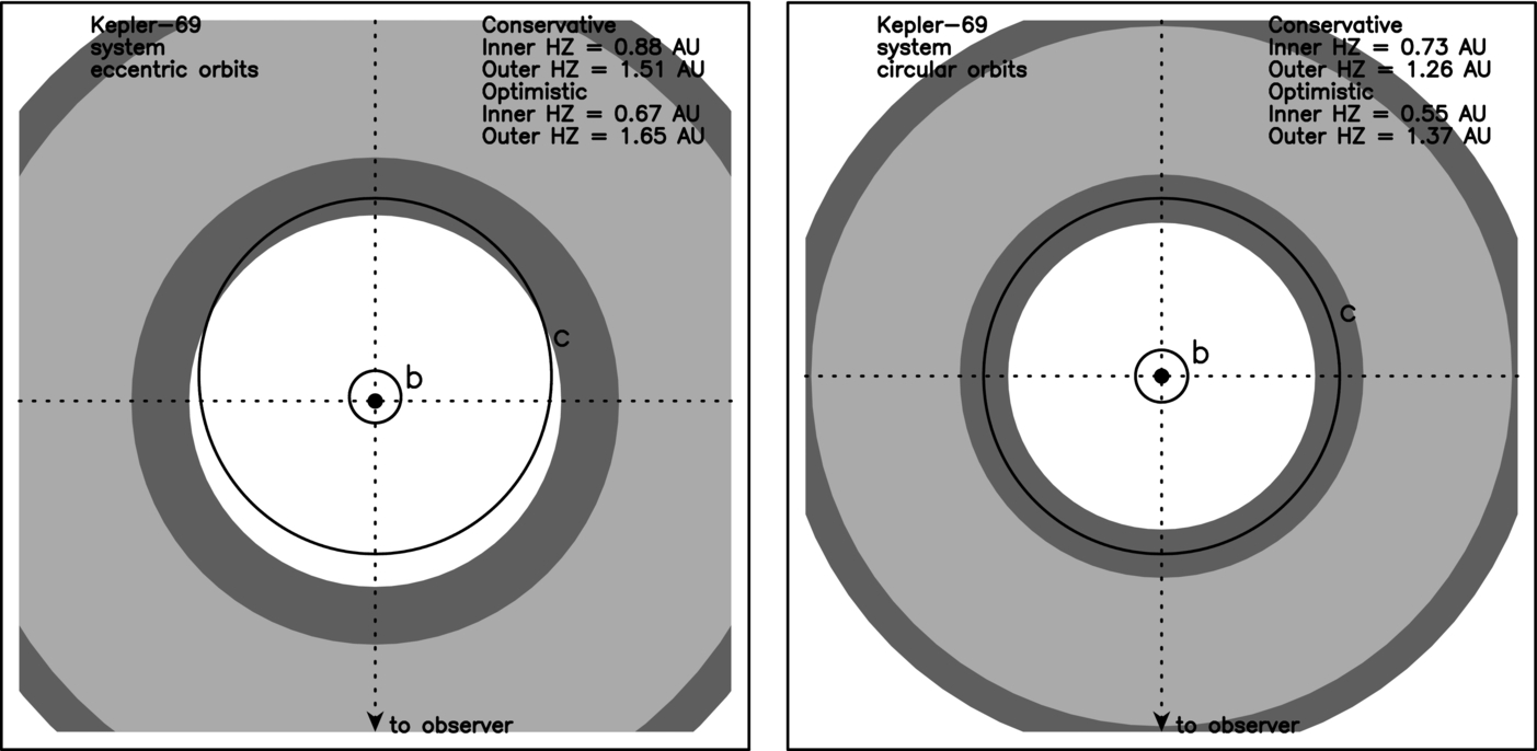
Figure 2 shows the orbits of the Kepler-69 planets overlaid on the calculated HZ regions for the star. The light gray represents the conservative regions and the dark gray regions represent the extensions to the HZ from the optimistic model. The left panel uses the stellar parameters and Barclay et al. (2013a) orbital solutions as shown in Table 1. The semimajor axes are 0.094 AU for planet b and 0.64 AU for planet c. For the conservative model, we calculate inner and outer HZ boundaries of 0.88 AU and 1.51 AU, respectively. For this model, neither planet ever enters the HZ. For the optimistic model, the inner and outer HZ boundaries are 0.67 AU and 1.65 AU, respectively. In this case, the apastron of the planet c orbit enters the HZ, assuming the eccentricity of 0.14 shown in Table 1. We calculate that 43.9% of the total orbital period is spent in the HZ where it is slowly moving through apastron. Planets in eccentric orbits which spend only part of their orbit in the HZ have been previously investigated (Kane & Gelino 2012c; Williams & Pollard 2002). These studies show that habitability is not necessarily ruled out. However, a grazing encounter with the optimistic inner boundary does not qualify the planet to be considered an "HZ planet" in this model.

Zoom In Zoom Out Reset image size

We further investigate a scenario which uses our MLE solution shown in Table 1 for both planets. We assume that the stellar parameters are 1σ lower than their measured values, thus we use an effective temperature and stellar radius of T_eff = 5470 K and R_* = 0.81 R_*, respectively. This results in the HZ moving inward slightly. For the conservative model, the inner and outer HZ boundaries are 0.73 AU and 1.26 AU, respectively. For the optimistic model, the inner and outer HZ boundaries are 0.55 AU and 1.37 AU, respectively. This scenario is depicted in the right panel of Figure 2, and shows that planet c may feasibly spend 100% of the orbit within the inner edge of the optimistic boundary. Recall that this uses the "Recent Venus" criteria (Kopparapu et al. 2013), which is empirically determined from an assumption that Venus once had surface liquid water but has been dry for at least the past 1 billion years (Solomon & Head 1991). If we adopt the unmodified stellar parameters, then planet c is always interior to even the optimistic HZ.

There are several intrinsic properties of the planet which may move the effective HZ closer to the star and thus encompass the planetary orbit. The first of these is the effect of clouds. As pointed out by Kopparapu et al. (2013), H₂O and CO₂ cloud effects are not included in their models since three-dimensional climate models are required. Attempts have been made to include specific cloud assumptions in HZ calculations, such as the work of Selsis et al. (2007). Scaling the results of Selsis et al. (2007) to the case of Kepler-69c is unlikely to be valid since they use a one-dimensional model which assumes an Earth-based atmospheric scale height which will certainly be different for the larger size of Kepler-69c. As shown by Forget & Pierrehumbert (1997), neglecting CO₂ clouds may result in an underestimation of the greenhouse effect. Generally speaking, the effect of H₂O clouds is to move the inner HZ boundary closer to the star but CO₂ clouds result in IR back-scattering, thus increasing the surface temperature and moving the HZ outward. Thus the extent to which the HZ boundary moves is sensitive to the underlying assumptions regarding the composition and convection of the planetary atmosphere.

A second property of the planet which may influence the extent of the HZ is the mass. Kopparapu et al. (2013) briefly address this aspect for Mars, Earth, and super-Earth (10 M_⊕) planets. In particular, they examine the effect of surface gravity which influences the column depth of the atmosphere and the subsequent strength of the greenhouse effect. Their results show that a larger surface gravity will move the inner edge inward, but a lower surface gravity will move the outer edge outward. The estimated radius of Kepler-69c is 1.71 R_⊕ (Barclay et al. 2013a). Using the stellar and planetary properties shown in Table 1 and the mass/radius/flux relationships of Weiss et al. (2013), we estimate a Kepler-69c mass of 2.14 M_⊕. This results in a density of ρ = 2.36 g cm⁻³ and a surface gravity of 0.73 times that of the Earth. This relatively low surface gravity implies that the mass and size of the planet will have little effect on the HZ and may in fact move the inner HZ boundary outward.

Finally, we note that Barclay et al. (2013a) address the issue of the HZ by calculating the equilibrium temperature of the planet based upon incident stellar flux and assumptions regarding the Bond albedo. As pointed out by Kopparapu et al. (2013), this approach is problematic since the albedo is wavelength dependent and may lead to discrepant values for the HZ boundaries. Our analysis here shows that Kepler-69c is unlikely to be in the HZ of the host star, although it is a good candidate to be confirmed as a super-Venus.

Considering that Kepler-69c has a similar orbital period to that of Venus, we consider here the possibility that the planet in fact may bear a Venusian surface environment at an increased scale. A particularly compelling consideration is that of the incident flux. The solar flux received by the Earth is approximately 1365 W m⁻² and the flux received by Venus is 2611 W m⁻², thus Venus receives 1.91 times more flux than the Earth. Kepler-69c receives a flux of 2614 W m⁻² from the host star which is also a factor of 1.91 times the flux received at Earth. This similarity in incident flux received between Venus and Kepler-69c is a primary motivator in discussing potential other similarities.

The relatively low density of the planet of ρ = 2.36 g cm⁻³ is similar to the Galilean moons of our solar system and indicates composition dominated by silicate and carbonate minerals rather than metals, consistent with the less than solar metallicity (Barclay et al. 2013a). Assuming that the planet formed in situ, it will have been subjected to water delivery during the late heavy bombardment, although it has been suggested by Morbidelli et al. (2000) that terrestrial planets can accrete significant water during formation without the need for cometary impacts. With such water delivery and a similar atmospheric evolution to Venus, the availability of silicates and carbonates in the crust of the planet may well have produced a thick CO₂ atmosphere and subsequent runaway greenhouse warming. In addition, the non-zero eccentric solution of Barclay et al. (2013a) will help to trigger further atmospheric changes via tidal heating (Barnes et al. 2013b). Thus a more likely scenario than a habitable super-Earth with liquid water is an inhospitable planetary surface with a thick CO₂ atmosphere, high temperatures, and high atmospheric pressure.

While developing techniques to characterize the planets that contribute to the η_⊕ population, such as photometric variability due to dynamic weather (Pallé et al. 2008), we can similarly determine how to distinguish these planets from those that comprise η_Venus. Although the Venusian surface is hot, the upper cloud layers are cool and so not necessarily a good indication of surface conditions. These clouds are also highly reflective, with a geometric albedo of 0.65 compared with 0.37 for the Earth. This means that a relatively large amplitude of reflected light (phase) variations for such planets may be a first indicator of a super-Venus in exosystems (Mallama 2009). In our own solar system, Venus is second only to Jupiter (43%) in the amplitude of the phase variations (Kane & Gelino 2013). In Figure 3 we show the calculated phase variations for the Kepler-69 system, including the effects of both planets for one complete orbital period of planet c. For this model, we have assumed a high Venusian geometric albedo and a very low albedo for the inner planet. Since the phase amplitude is proportional to $R_p^2/a^2$, the inner planet will overwhelmingly dominate the phase signature. Even so, the phase amplitude of planet c is ∼3.5 times higher than Venus and thus may be a useful diagnostic in similar systems. Note that the geometric albedo and therefore the phase amplitude has a strong wavelength dependence.

Zoom In Zoom Out Reset image size

A more robust method is to measure the major atmospheric components via transmission spectroscopy (Hedelt et al. 2013). The atmospheric signature of Venus has been extensively studied, and further opportunities via the recent 2004 and 2012 transits have been exploited to great effect (Hedelt et al. 2011). It is well established that Earth and Venus have many differences between their transmission spectra, the most prominent being due to the type of scattering that dominates in the UV and optical wavelengths (Ehrenreich et al. 2012). For Earth, Rayleigh scattering is the dominant effect, whereas for Venus it is Mie scattering in the cloud and haze layers that influences the shape of the spectral continuum.

Another signature of the Venusian atmosphere is the identification of the CO₂ dominant atmosphere. In emission spectra, CO₂ features emission peaks at 4.3 and 15 μm due to the atmospheric temperature inversion (Hedelt et al. 2013). Observations of atmospheric abundances at low altitudes is difficult for Venus since H₂SO₄ clouds are optically thick and obscure the lower atmosphere (Schaefer & Fegley 2011; Ehrenreich et al. 2006). However, because of the very different temperature structures of the Earth and Venus atmospheres, the CO₂ show significant differences in transmission spectra. As mentioned earlier, the Venusian upper atmosphere is efficiently cooled due to the strong greenhouse effect trapping the IR radiation at the surface. Thus, a lack of detectable IR CO₂ emissions in the upper atmosphere may indicate the presence of a greenhouse closer to the surface which renders the planet uninhabitable. The detectability of such signatures has been investigated by Ehrenreich et al. (2012) and found to be feasible with planned instrumentation for the James Webb Space Telescope (JWST) and the European Extremely Large Telescope, although ground-based detection of CO₂ bands is rendered nearly impossible due to the strong presence of the molecule in our own atmosphere. Even so, there are indeed future instrumentation opportunities that will remove the ambiguity when attempting to distinguish between super-Earth and super-Venus atmosphere analogs.

The extraordinary diversification of the exoplanetary field is enabling us to finally place our solar system in context. The frequency of Jupiter analogs and Earth analogs are key components to understanding the precise nature of that context. However, as the sensitivity of current detection techniques reaches into the terrestrial-size regime, we also need to be able to distinguish between Earth and Venus analogs in order to place our habitability in context. Thus, the key question of how common Earth-like planets are relies on also understanding how frequently terrestrial planets diverge into Venusian-type evolutionary pathways which may place heavy constraints upon habitability prospects. The Kepler mission is already revealing many planets which fall into the terrestrial-size planetary regime and, as we have shown here, there are cases where the properties of the system straddle current HZ boundary calculations. The case of the Kepler-69 system is particularly interesting because the host star is only slightly less massive than our own Sun, thus providing an easier comparison to the HZ and planets or our solar system. It is a considerable hindrance to our studies of larger-than-Earth terrestrial planets that our system contains no such objects. However, considering the high occurrence rate of these types of planets, it is likely that these will dominate exoplanet atmospheric studies well into the next decade. Atmospheric characterization of large terrestrial planets has a productive future ahead of it with the anticipated discoveries of the Transiting Exoplanet Survey Satellite and subsequent follow-up with the JWST. The detection of Venusian-type atmospheres at a variety of orbital periods and planetary masses will create a picture of where the divergence between Earth and Venus originates.

The authors would like to thank David Ciardi, Lauren Weiss, and the anonymous referee for productive feedback. This work has made use of the Habitable Zone Gallery at hzgallery.org.