

Abstract
Coastal slope is a fundamental land characteristic that can influence the hydrodynamic and morphological processes, which is the essential parameter to calculate the wave setup and wave run up for further estimating extreme coastal water levels. Slope information of coastal zones also plays a key role in estimating the coastline erosion and evaluating the coastal vulnerability under sea level rise. However, accurate estimates of coastal slopes are currently limited, especially over sparsely populated and remote areas. The recent ICESat-2 photon-counting lidar provides unprecedented along-track dense and accurate height measurements in coastal zones. This study aims to demonstrate the potential of ICESat-2 measurements to estimate coastal slope of sandy beach at a large scale, and the proposed method is tested in Texas, USA. The validation with local airborne lidar data (with an average slope of 0.023 in Texas) indicates that, the ICESat-2 derived coastal slopes (0.026) have much better accuracy than current large-scale coastal slopes (0.0032) derived from SRTM and MERIT DEMs. With globally covered ICESat-2 datasets, this method can be expanded to estimate coastal slopes even at a global scale.
Export citation and abstract BibTeX RIS

Original content from this work may be used under the terms of the Creative Commons Attribution 4.0 license. Any further distribution of this work must maintain attribution to the author(s) and the title of the work, journal citation and DOI.
1. Introduction
As an important transitional area between ocean and land, the coastal zone supports complex ecosystems with rich biodiversity (Maune and Nayegandhi 2007, Bosnic et al 2017). Exceeding 40% of the global population lives in areas within 200 km to the coastline (Jouffray et al 2020), and 70% of the industrial capital is located within the coastal zone 100 km from the coastline (Zong et al 2021). Under the double pressure of climate change driven sea level rise and disturbance of human activities, accurate geographical information is urgently required for sustainable management in coastal zones (He and Silliman 2019, Kulp and Strauss 2019, Xu et al 2022a).
Coastal slope is a fundamental land characteristic that can influence the hydrodynamic and morphological processes, which is the essential parameter to calculate the wave setup and wave run up for further estimating extreme coastal water levels (Almar et al 2021). Slope information of coastal zones also plays a key role in evaluating coastal vulnerability, which can be caused by sea level rise, coastal erosion, storm surge flooding, saltwater intrusion into groundwater aquifers, or inundation hazards (Gornitz et al 1994, Shaw et al 1998, Hammar-Klose and Thieler 2001, Pendleton et al 2005, 2010a, Stockdon et al 2007, Senechal et al 2011, Tano et al 2016, Athanasiou et al 2019, Befus et al 2020). Meanwhile, accurate coastal slope information is also essential for coastal resource use, coastal ecosystem protection, and sustainable development in coastal zones (Maestro et al 2019, Popova et al 2019).
Currently, coastal slope can be calculated from regularly spaced transects perpendicular to the coastline that are obtained by global navigation satellite system devices, or calculated from the coastal topography that is generally obtained by airborne lidars. Doran et al (2015) used the lidar points and endpoint method to calculate the spatially and temporally averaged beach slope and estimate the uncertainty. Nijland et al (2017) used a lidar-based terrain model to estimate slope information near the coastline. Taramelli et al (2020) combined the field spectral library, airborne hyperspectral imagery, topographic/bathymetric lidar derived digital surface model and bathymetric position index to obtain slope information in coastal zones. With locally measured datasets, these approaches provide estimates characterized by high accuracy and resolution but by low coverage, especially over remote areas.
Using large-scale topographic and bathymetric products, e.g. SRTM30/SRTM90 (Shuttle Radar Topography Mission) at 30/90 m resolution and General Bathymetric Chart of the Oceans at 900 m resolution), previous studies made a great achievement in estimating coastal slopes at regional and even global scale (Hammar-Klose and Thieler 2000, Divins and Metzger 2009, Pendleton et al 2010b, Athanasiou et al 2019, Diaz et al 2019). The resolution of several tens of meters in global DEMs and bathymetric charts may have an impact on the accuracy of the derived slopes. Specifically, based on the satellite imagery-based on shoreline positions and frequency domain analysis, Vos et al (2020), (2022) proposed a novel method to estimate coastal slope with a very high accuracy and obtained regional coastal slope dataset at California, USA and Australia.
The new generation spaceborne photon-counting lidar borne on NASA's Ice, Cloud and land Elevation Satellite-2 (ICESat-2) may assess the coastal slope estimation at a large scale with a high accuracy. ICESat-2 has one laser that is split into six laser beams (i.e. three strong laser beams and three weak laser beams with a transmitted energy ratio of 4:1). With a laser repetition rate of 10 kHz and an average flight altitude of 500 km, the adjacent laser footprint spacing is only 0.7 m in the along-track direction (Markus et al 2017, Martino et al 2019, Neuenschwander and Magruder 2019). With a footprint diameter of approximately 11 m, the geolocation accuracy and ground surface precision of ICESat-2 measurements are approximately 3.5 m (Magruder et al 2021) and 0.1–0.2 cm (Brunt et al 2019, Tian and Shan 2021), respectively. With high-sensitivity photon-counting detectors and a green 532 nm laser, ICESat-2 can obtain seafloor reflected signal at the depth exceeding 30 m with an accuracy of ∼0.5 m in very clear waters (Parrish et al 2019, Ma et al 2020, Babbel et al 2021, Thomas et al 2021, Xu et al 2022b). Benefitting from these advantages, ICESat-2 can unprecedentedly obtain six surface profiles along the reference ground tracks (RGTs).
Using the global coverage datasets of ICESat-2, some studies have investigated methods to obtain coastal topographic information, e.g. Xie et al (2021) proposed a method based on spatial statistical features of captured photons. Liu et al (2022) combined ICESat-2 derived surface profiles and Sentinel-2 derived spectral features to identify land cover types in coastal zones. ICESat-2 data has exhibited a great potential in reflecting coastal slope or topography due to its high vertical accuracy, dense point cloud along the ground track. In this study, using ICESat-2 datasets, we propose a method to estimate coastal slopes of sandy beach at a regional scale. We use the coast of the state of Texas, USA as a case study, where the coastal type is dominated by sandy beaches. With local measurements as the reference data, the derived results are validated, which demonstrates its performance and potential in obtaining reliable coastal slopes. We further use the generated coastal slopes to evaluate the coastal vulnerability near Texas coast as one case of possible future applications for this new method.
2. Materials
2.1. Definition and global extension of sandy beaches
The width of sandy beach is defined as the distance between the dune toe and coastline along the cross-shore profile, and the slope of sandy beach is normally calculated using the beach width and the elevation difference between the coastline and dune toe. Here, the sandy beach is selected in this study with the following reasons. (1) In different coastal types (bedrocks, sandy beaches, tidal flats, and artificial coasts), sandy beaches are highly dynamic in time and space and constitute an important part of the world's coastline (Çelik and Gazioğlu 2022). Luijendijk et al (2018) indicate that 31% of the world's ice-free coastline are sandy beaches. (2) This method is applied to sandy beaches also because of its topography characteristics. In remote areas where direct assessments are not possible, compared with the other two natural coasts (i.e. bedrocks and tidal flats), sandy beaches are generally characterized by relatively consistent and gentle slopes from the coast to land. The slope of bedrocks is difficult to define due to their irregular surfaces, whereas tidal flats normally have lower slopes and many of tidal flats submerge with high tide level. For artificial coasts, many direct assessments are available. (3) The relatively consistent and gentle slope of sandy beaches favor the usage of the ICESat-2 lidar for topographic assessments, which has a footprint diameter of ∼11 m with the geolocation accuracy of several meters and the ground surface precision of tens of centimeters (Magruder et al 2021, Tian and Shan 2021).
2.2. Study area and satellite data
Texas coast in the northwest Gulf of Mexico is selected as the study area in figure 1. Texas coast has only one high and low tide every day (i.e. the diurnal tide) and is with a tidal range of approximately 2 m (https://oceanservice.noaa.gov/education/tutorial_tides/tides07_cycles.html). Near Texas coast, the Mississippi River brings a large amount of sediments into the bay, forming a huge estuary delta and large underwater alluvial fan (Nittrouer and Viparelli 2014). Texas has approximately 599 km of open bay shoreline (Mao et al 2022), which is dominated by narrow muddy and sandy beach (https://tpwd.texas.gov/business/grants/wildlife/cwcs/media/docs/coastal/coastal_final.doc). Coastal wetlands in Texas include intertidal saline marshes, seagrass, and mangroves. Texas coast has been eroded severely (Hutchison et al 2018) and has one of the highest subsidence rates in the world, with the long-term rate of 0.05 mm yr−1 (Paine 1993). According to sea level observation data of seven tidal stations (red points in figure 1) along the Texas coast, regional sea level rise with a rate of ∼4.92 mm yr−1 (https://tidesandcurrents.noaa.gov/sltrends/sltrends.html) from 1984 to 2016 and was ∼1.89 mm yr−1 faster than the global average sea level rise rate (www.star.nesdis.noaa.gov/socd/lsa/SeaLevelRise/LSA_SLR_timeseries_global.php).
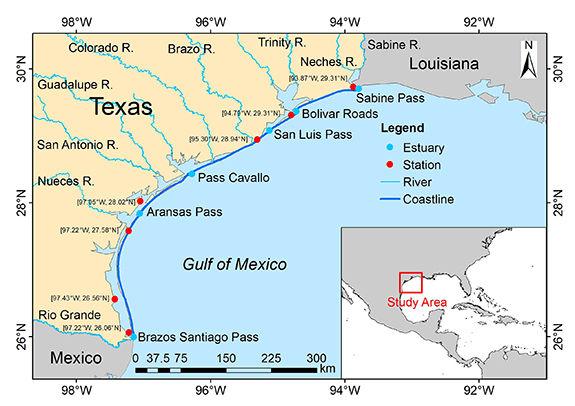
Figure 1. Map of the study area (Texas, USA). In this map, six estuaries (Sabine Pass, Bolivar Roads, San Luis Pass, Pass Cavallo, Aransas Pass, and Brazos Santiago Pass from north to south) are marked by light blue dots, and seven tidal stations (Sabine Pass, Galveston Pier, Freeport, Rockport, Corpus Christi, Port Mansfield, and Port Isabel from north to south) are marked by red dots. The dark blue line shows the outer sandy coastline connected to the open sea, and the light blue curves show the centerlines of main rivers in Texas, USA. In the inset, the red box shows the geographical location of our study area.
Download figure:
Standard image High-resolution image2.3. Datasets
In the study area, 729 ICESat-2 ATL03 datasets and 397 ICESat-2 ATL08 datasets from September 2018 to July 2021 are used to estimate the slope of sandy beach. In other words, ICESat-2 has passed over the study area for 729 times during 2018–2021. However, some of these ATL03 729 datasets do not contain signal points on the ground (i.e. sandy beach in this study) as the cloud and fog frequently occur near the coast, which sharply attenuates the laser energy and prevents the laser pulse reaching the ground. ICESat-2 has one laser that is split into six laser beams, in that ICESat-2 can obtain six surface profiles along the RGTs. Considering the cloud and fog as well as other impacts, in this study, 713 coastal slope transects perpendicular to the directions of the Texas coastline are calculated from 713 valid ground tracks in all available ATL03/ATL08 datasets.
The ATL03 product contains geolocated photons of six ground tracks, and each photon has its time tag, longitude, latitude, elevation (with respect to the WGS84 ellipsoid), confidence level, and other information (Neumann et al 2021). The geolocated photons in the ATL03 product have implemented geophysical corrections (i.e. the geoid, ocean tides, atmospheric correction) (Markus et al 2017). These geolocated photons in the ATL03 product include signal points and noise points (mainly due to the solar background). With an effective signal point detection method, the signal points on the ground (which are detected from these geolocated photons) have an elevation uncertainty of ∼0.2 m for plain terrain (Tian and Shan 2021) and ∼0.14 for icesheet (Brunt et al 2019).
The confidence level in the ATL03 product provides a preliminary classification for each photon as either a likely signal photon or noise (Neumann et al 2019). For land areas, a more reliable signal finding method of differential, regressive, and Gaussian adaptive nearest neighbor is used in the ATL08 product (Neuenschwander and Pitts 2019), which effectively searches the possible signal photons in the ATL03 product and provides the category tags as 'noise', 'ground', 'canopy', and 'top of canopy' photons (Neuenschwander et al 2021). Based on the RGT number, the ATL03 product can be linked with its corresponding ATL08 product. Note that some ATL03 datasets do not have their corresponding ATL08 datasets, which may be caused by that no signal photons are found or the RGT is not on land areas. As a result, in the study area, only 397 ICESat-2 ATL08 datasets are available, the number of which is much less than that of the ATL03 datasets (729). In practice, with the assistance from the ATL08 product, we can quickly find the valid ATL03 product in land areas.
According to Texas coastline data available in https://mapcruzin.com/, we manually determine the coastline of sandy beach using ArcGIS. In this study, we conduct comparisons from two respects. First, we compare our derived slopes of sandy beach in Texas with a local slope dataset derived from a United States Geological Survey (USGS) high-resolution airborne lidar (https://coastal.er.usgs.gov/data-release/doi-F7GF0S0Z/), which is to evaluate the accuracy and consistency of our result. The local dataset from USGS contains dune crest, dune toe, and coastline at a 10 m resolution (Doran et al 2020). For each coastline location, this local dataset also provides the beach width and beach slope from the dune toe to the coastline. Unfortunately, the used USGS airborne lidar data were acquired over 2018–2019, which is earlier than the acquisition time of ICESat-2 data over 2018–2021.
Second, we compare our derived slopes with the global coastal slope product from Athanasiou et al (2019) to demonstrate the advantage of our result at a large scale. The coastal slope from Athanasiou et al (2019) was derived from the two global datasets, i.e. (1) the MERIT digital elevation model (DEM) (http://hydro.iis.u-tokyo.acjp/~yamadai/MERIT_DEM/), which is an improved version of the existing spaceborne DEMs SRTM3 v2.1 and AW3D-30 m v1 products at 90 m resolution; and (2) the General Bathymetric Chart of the Oceans (www.gebco.net) at 900 m resolution.
3. Methods
To assess the coastal slope along Texas coast, we propose a method that combines ICESat-2 ATL03 and ATL08 products. Figure 2 illustrates the schematic diagram of the calculation process. First, linking the ATL03 product with its corresponding ATL08 product using the RGT number, we can directly extract the time tags, longitudes, latitudes, elevations of all signal photons with the ATL08 'ground' tags. The extracted signal photons on the ground are the preliminary signal data in this study. In relatively flat ground surfaces, the interval between these signal photons can reach 0.7 m in the along-track direction, i.e. each laser shot has at least one signal photon especially for the strong beam. Note that the ATL08 'ground' photons may contain signal photons on the sea surface.

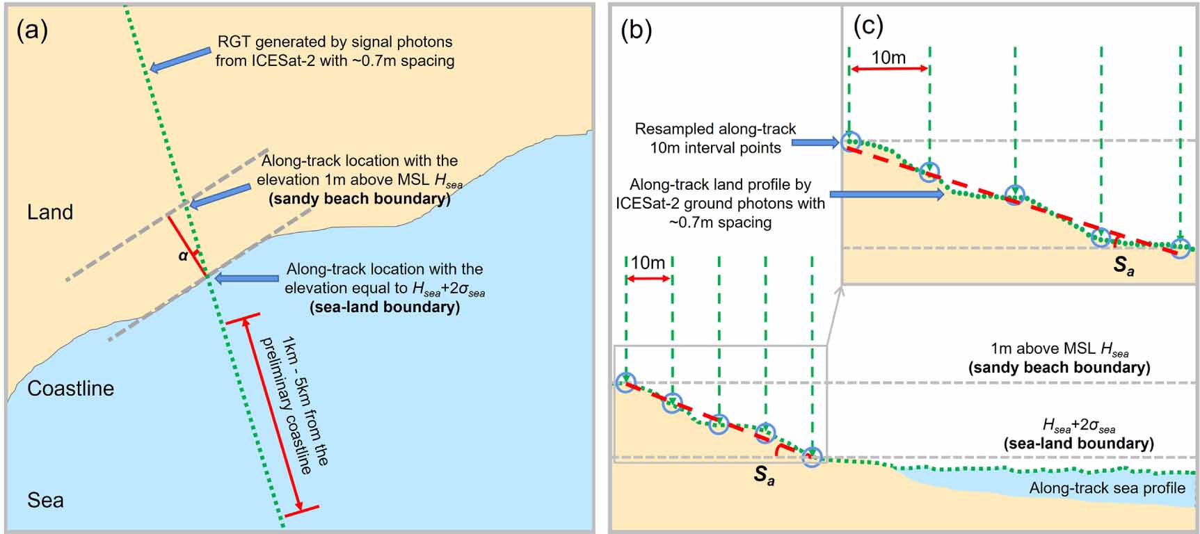
Figure 2. (a) Top view of an ATL03/ATL08 ascending ground track (the green dotted line) intersecting the coastline (the grey solid curve). (b) Side view of the profile of the land and sea surface. (c) Enlarged area of the gray box in (b). Note that we use 1 m above the mean sea level (MSL) as the maximum height to estimate coastal slopes because the most estimate of global mean sea-level rise within this century falls below 1 m (Oppenheimer et al 2019).
Download figure:
Standard image High-resolution imageSecond, we discard the possible sea surface photons and determine the signal photons on the sandy beach. According to the coastline of Texas from https://mapcruzin.com/, for each ATL03/ATL08 ground track, only the extracted signal photons within 5 km along-track distance to the preliminary sea-land boundary (or coastline) are retained. Considering the tidal effect, for each track, the remaining signal photons on the sea side within 5 km to 1 km to the coastline are identified as sea surface photons, which are used to calculate the local mean sea level (MSL) Hsea (i.e. the average elevation) and the wave height σsea (i.e. the standard deviation). The along-track location with the elevation equal to Hsea + 2σsea is determined as the sea-land boundary (or coastline) considering the tidal effect, and only signal photons on the land side are retained. Then, the along-track location with the height of 1 m above the MSL is found and determined as the sandy beach boundary (Oppenheimer et al 2019). In other words, only the signal photons in the along-track segment with elevations ranging from Hsea + 2σsea to 1 m above the MSL are retained and used as ground points of the sandy beach to estimate the slope information.
We use ground photons within only 1 m elevation range mainly based on the Intergovernmental Panel on Climate Change (IPCC) 2019 report (Oppenheimer et al 2019). Specifically, if countries significantly reduce emissions (Representative Concentration Pathways, RCP2.6), the IPCC expects 0.35–0.60 m of the global sea level rise in 2081–2100 relative to 1986–2005. Under the high emission scenarios (RCP8.5), the IPCC projects 0.60–1.05 m of the global sea level rise in 2081–2100 relative to 1986–2005 (or approximately 15 millimeters per year). Under any scenarios, the global sea level rise by 2100 is within 1.05 m compared to current MSL. As a result, the ground photons of ICESat-2 with 1 m elevation range, i.e. from current local MSL to 1 m above MSL, are selected to derive the coastal slope. In addition, a small elevation range of 1 m, we can simultaneously discard the possible influence from coverings on the sandy beach (e.g. artificial objects, shrubs, and rocks).
Third, for ground points within the sandy beach in each ground track, we resample the along-track point interval to 10 m as shown in figures 2(b) and (c) using blue circles. Specifically, for each 10 m along-track segment step-by-step starting from the coastline, we calculate the average elevation (Hbeach) and the standard deviation (σbeach) of these approximately 0.7 m spacing ground points. In each 10 m interval, the ground points whose elevations are beyond Hbeach± 2.5σbeach are filtered out, and the average elevation of the remaining ground points in each 10 m along-track segment is calculated as the filtered elevation.
Next, using the robust linear regression, the slope Sa along the ICESat-2 ground track is estimated using the 10 m re-sample points. The ICESat-2 ground track may not be perpendicular to the coastline. As a result, we further calculate the angle α between the ground track direction and the normal direction of the coastline as shown in figure 2(a). The slope of the sandy beach Sp in the direction perpendicular to the coastline is then corrected as Sp = Sa /cosα. Finally, to evaluate the method performance, the coastal slopes generated from USGS airborne lidar are used as the in-situ measurements. Here, the root mean square error (RMSE) and correlation coefficient (r) are calculated to quantify the accuracy and consistency between the ICESat-2 derived coastal slopes and in-situ measurements.
4. Results
Using ICESat-2 ATL03 and ATL08 products, this study obtains the coastal slope results of sandy beach in Texas, USA. Along the 599 km coastline of Texas, beach coastline is ∼581 km, accounting for ∼97% (Mao et al 2022). In figures 3(a) and (b), 713 coastal slope transects perpendicular to the directions of the coastline are calculated from 713 valid ground tracks in 397 ATL03/ATL08 datasets. In these 713 valid ground tracks, the average elevation range of the selected signal photons within sandy beach (that are used to estimate the slope) is 0.86 m, and the average along-track distance from the sandy beach boundary to coastline is 74.26 m.

Figure 3. (a) Derived coastal slope results in the study area (i.e. Texas, USA). (b) Percentages of different coastal slopes. (c) Comparison between the coastal slopes derived from ICESat-2 (mean: 0.026) and airborne lidar data (mean: 0.023). (d) Comparison between coastal slopes from the study of Athanasiou et al (2019) (mean: 0.0032) and airborne lidar data (mean: 0.023).
Download figure:
Standard image High-resolution imageAs shown in figures 2(b) and (c), the coastal slope is estimated by inputting the 10 m resampled points (blue circles) into the robust linear regression algorithm. The average residuals (Re) and determination coefficients (R2 ) between the regression results and 10 meters resampled points are listed in figure 3(a) for six different ranges of the derived slopes in Texas (i.e. <0.02; 0.02–0.03; 0.03–0.04; 0.04–0.05; 0.05–0.10; >0.1). In total, for these coastal slopes derived from their corresponding robust linear regression models, and the average R2 (the determination coefficient) is 0.96, and the number with statistical significance (p < 0.05) is 698, accounting for 98% of all 713 models. The values of Re and R2 indicate that the regression results are consistent with the actual observations of ICESat-2, which indicates the derived coastal slopes are reliable.
The derived slopes in the study area indicate an obvious spatial heterogeneity. Six estuaries (red lines in figure 3) are used to divide the coast of Texas into five coastal units. From the mouth of the Mississippi River to the border between Mexico and the United States, the average slopes of five coastal units are 0.024 (with 151 derived slope transects), 0.021 (62), 0.027 (349), 0.021 (66), and 0.028 (85), respectively.
From figures 3(c) and (d), our derived coastal slopes are validated with the USGS airborne lidar data-derived slopes, which exhibits much better performance (RMSE = 0.009, r= 0.58, p < 0.05) compared with a previous global coastal slope dataset obtained by Athanasiou et al (2019) (RMSE = 0.025, r = −0.13, p > 0.05). As illustrated in figure 3(c), the correlation coefficient (r = 0.58) mainly suffers from the differences when ICESat-2 derived relatively larger slopes, and some potential reasons as follows. First, the used airborne lidar data-derived coastal slope dataset is a re-analysis dataset with a 10 m resolution near the coastline (Doran et al 2020) rather than the direct field measurements. Also, the airborne lidar data were acquired over 2018–2019 while the ICESat-2 data were acquired over 2018–2021, which inevitably introduce errors and may be the main error source. Second, in figure 3(a), with steeper slopes (>0.1), the average R2 are still close to 1 but the average residual Re (with a mean of 0.17 m) is much larger than that of lower slopes (with a mean Re less than 0.04 m when the derived coastal slopes are <0.1). A larger residual Re indicates some fluctuations exist in sandy beach, which may introduce error when estimating the coastal slope.
5. Discussion
In this section, we employ the derived slopes to assess Texas's coastal vulnerability index (CVI) under sea level rise, which is one case of possible future applications for this new method and its derived coastal slope dataset. Coastal slope is an important factor in assessing coastal vulnerability, and USGS specifically considers six variables in evaluating coastal vulnerability, i.e. the geomorphology, shoreline change rate, coastal slope, relative sea level rate, mean significant wave height, and mean tidal range. The CVI was originally proposed by Gornitz and Kanciruk (1989) as an important measure of the likelihood of physical changes in the coastline due to sea level rise. The global applicability of CVI was demonstrated by Gornitz (1991), Thieler and Hammar-Klose (2000), Pendleton et al (2005, 2010a), Tano et al (2016), and Neelamani et al (2021).
The CVI score can be calculated as
where a is the geomorphology of coastline types, e.g. the sandy beach dominates coastline type in Texas (Mao et al 2022); b is the shoreline change rate (m yr−1), which is available from Luijendijk et al's study (2018); c is the coastal slope, which is derived from ICESat-2 in this study; d is the relative sea-level change (mm yr−1) available on https://tidesandcurrents.noaa.gov/sltrends/sltrends.html; e is the mean significant wave height (m) available on https://marine.copernicus.eu/; and f is the mean tidal range (m) available on https://tidesandcurrents.noaa.gov/sltrends/sltrends.html.
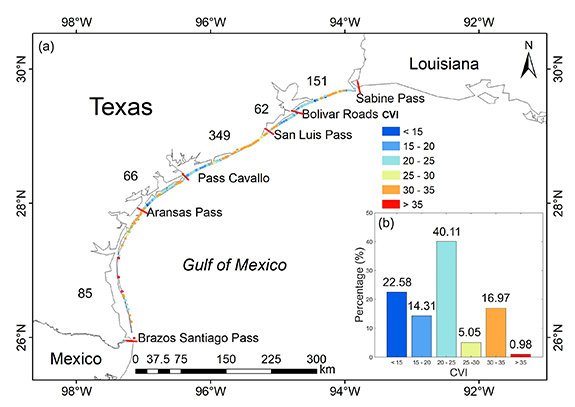
The CVI scores are divided into low, moderate, high, and very high risk categories (Thieler and Hammar-Klose 1999, Kantamanenia et al 2018, Tano et al 2018). Specifically, CVI values below 15 are assigned to the low risk category, values from 15–20 are considered as moderate risk, values from 20–25 are considered as high risk, and values above 25 are considered as very high risk. Figure 4(a) illustrates the derived spatial distributions of CVI scores in Texas, whereas figure 4(b) indicates that the low risk category accounts for 22.58%, the moderate risk accounts for 14.31%, high risk accounts for 40.11%, and very high risk accounts for 23%. More than half of the Texas coast faces high risk under sea level rise (i.e. CVI > 20).
Figure 4. (a) Calculated coastal vulnerability index (CVI) spatial distributions in Texas; (b) percentages of different CVIs.
Download figure:
Standard image High-resolution image
In addition, the new method and its derived coastal slope dataset in this study can also be used to model coastal erosion under sea level rise in the future. The coastal slope information is the key parameter in the classic and modified Bruun rule (Bruun 1962, Bird 1996, Cooper and Pilkey 2004, FitzGerald et al 2008, Le Cozannet et al 2016, Mentaschi et al 2018, Wright et al 2019). The Bruun rule has been widely used to quantify the relationship between sea level rise and coastline erosion for sandy beach. According to the Bruun rule, sea level rise is one of the important drivers for sandy coastline retreat (Gibeaut et al 2000, Paine et al 2017) and barrier chain deterioration (Williams et al 1992, FitzGerald et al 2008).
6. Conclusions
In this study, we develop a method for generating coastal slopes of sandy beach using ICESat-2 ATL03 and ATL08 products, and this method is validated in the coastal zone of Texas, USA. In the study area, the mean and the standard deviation of coastal slopes are 0.025 and 0.022, and in the regression model, the average R2 is 0.96 with 98% statistically significant estimation. In the validation between our derived coastal slopes and the local airborne lidar data-derived slopes, the RMSE and correlation coefficient are 0.009 and r = 0.58, respectively. The coastal vulnerability near Texas coast is evaluated as one case of possible future applications for this new method and its derived coastal slope dataset, and the results indicate more than half of the Texas coast faces high risk under sea level rise (i.e. CVI > 20). On one hand, this regional-scale accurate coastal slope dataset is very fundamental to improve the coastline change estimation, coastal vulnerability assessment, and regional coastal map update in Texas under global warming driven sea level rise. On the other hand, with globally covered and freely accessed ICESat-2 datasets, this method can be expanded to generate the coastal slope in many other regions or even at a global scale.
Acknowledgments
This research was funded by the National Natural Science Foundation of China Grant 42101343 to N X; Natural Science Foundation of Shandong Province, China Grant ZR2020MD022 to Y M; Hubei Provincial Key Research and Development Program, China Grant 2022BID6 to S L. We thank the NASA National Snow and Ice Data Center (NSIDC) for distributing the ICESat-2 data (https://doi.org/10.5067/ATLAS/ATL03.004 and https://doi.org/10.5067/ATLAS/ATL08.004) and the United States Geological Survey (USGS) for distributing high-resolution airborne lidar data (https://coastal.er.usgs.gov/data-release/doi-F7GF0S0Z/). We thank the website https://mapcruzin.com/ for providing Texas coastline data, https://tidesandcurrents.noaa.gov/sltrends/sltrends.html for providing Texas sea-level change rate and mean tidal range data, and https://marine.copernicus.eu/ for providing Texas significant wave height data.
Data availability statement
The ICESat-2 ATL03 and ATL08 products in this study are available on the NSIDC website (https://doi.org/10.5067/ATLAS/ATL03.004 and https://doi.org/10.5067/ATLAS/ATL08.004). The in-situ slope dataset from United States Geological Survey (USGS) is available on https://coastal.er.usgs.gov/data-release/doi-F7GF0S0Z/. The Texas coastline data are available on and https://mapcruzin.com/, the Texas sea-level change rate and mean tidal range data are available on https://tidesandcurrents.noaa.gov/sltrends/sltrends.html, and the Texas significant wave height data are available on https://marine.copernicus.eu/.
The data that support the findings of this study are openly available at the following URL/DOI: https://zenodo.org/record/6498182#.Ymlf4shZFB5.