

Abstract
The Greenland high (GL-high) coincides with a local center of action of the summer North Atlantic Oscillation and is known to have significant influence on Greenland ice sheet melting and summer Arctic sea ice. However, the mechanism behind the influence on regional Arctic sea ice is not yet clear. In this study, using reanalysis datasets and satellite observations, the influence of the GL-high in early summer on Arctic sea ice variability, and the mechanism behind it, are investigated. In response to an intensified GL-high, sea ice over the Beaufort Sea shows significant decline in both concentration and thickness from June through September. This decline in sea ice is primarily due to thermodynamic and mechanical redistribution processes. Firstly, the intensified GL-high increases subsidence over the Canadian Basin, leading to an increase in surface air temperature by adiabatic heating, and a substantial decrease in cloud cover and thus increased downward shortwave radiation. Secondly, the intensified GL-high increases easterly wind frequency and wind speed over the Beaufort Sea, pushing sea ice over the Canadian Basin away from the coastlines. Both processes contribute to an increase in open water areas, amplifying ice–albedo feedback and leading to sea ice decline. The mechanism identified here differs from previous studies that focused on northward moisture and heat transport and the associated increase in downward longwave radiation over the Arctic. The impact of the GL-high on the regional sea ice (also Arctic sea ice extent) can persist from June into fall, providing an important source for seasonal prediction of Arctic sea ice. The GL-high has an upward trend and reached a record high in 2012 that coincided with a record minimum summer Arctic sea ice extent, and has strong implications for summer Arctic sea ice changes.
Export citation and abstract BibTeX RIS

Original content from this work may be used under the terms of the Creative Commons Attribution 4.0 license. Any further distribution of this work must maintain attribution to the author(s) and the title of the work, journal citation and DOI.
1. Introduction
In the context of amplified Arctic warming, summer Arctic sea ice has decreased in extent and thinned rapidly in recent decades. While it is recognized that the disappearing sea ice directly follows the anthropogenic global warming [1], the processes that control the interannual variations of Arctic sea ice are still not well understood.
Numerous studies have suggested that the atmospheric circulation patterns in northern mid-to-high latitudes have contributed largely to the interannual as well as the long-term variations in Arctic sea ice through dynamic and thermodynamic processes [2–7]. These patterns include the Arctic Oscillation (AO), North Atlantic Oscillation (NAO), Arctic dipole (AD) and the Greenland anticyclone (hereafter, in short Greenland high or GL-high). Recent studies indicate that the localized circulation patterns are mostly relevant to Arctic sea ice variability. The AD pattern, defined as the second-leading mode of monthly sea level pressure, and the AD-wind pattern, derived from wind vector variability, are both suggested to have contributed significantly to the recent summer Arctic sea ice extent minima [7–9]. The positive phase of the AD pattern is characterized by high pressure anomalies over the North America side and low pressure anomalies over northern Siberia [6, 7], but with some variations depending on the analysis period used. Thermodynamically, the AD pattern can enhance water vapor and heat transport from lower and mid-latitudes to the Arctic [10–12], which favors enhanced convergence of the energy flux and increased downward longwave radiation (DLR) [13–15]. Dynamically, the AD pattern is associated with a strong surface pressure gradient across the Fram Strait that can enhance wind-driven transport of sea ice out of the Arctic Ocean and into the North Atlantic [7, 16]. The GL-high is characterized by a blocking pattern and a strong anticyclone over Greenland. Variations in the GL-high mostly resemble the summer NAO, but emphasizing local circulation changes [17]. It is known that the AD pattern is also correlated with the GL-high in early summer [10].
Based on statistical analysis and model experiment, it is found that anticyclonic circulation over Greenland and the Arctic Ocean has a positive trend with increased DLR, contributing up to 60% of the September sea-ice extent (SIE) decline since 1979 [2]. Overall, the mechanism behind the impacts of AD or GL-high has been largely associated with anticyclonic circulation and DLR [2, 5]. However, we know that anticyclonic circulation is often accompanied by subsidence and cloudless conditions, potentially resulting in increased downward shortwave radiation [18, 19]. Such effects remain to be clarified.
2. Data and methods
2.1. Data
Monthly mean sea ice concentration (SIC) for the period of 1980–2019 is obtained from the National Snow and Ice Data Center (NSIDC). This dataset is derived from Special Sensor Microwave Imager/Sounder on board the Defense Meteorological Satellite Program satellites using the NASA team algorithm [20]. The data are provided on the equal-area scalable Earth (EASE)-grid with a spatial resolution of 25 km. Monthly SIE is obtained from the NSIDC, which is defined as the total area covered by at least 15% SIC. Monthly sea ice motion is obtained from the similar 25 km Polar Pathfinder EASE-grid archived by NSIDC. Three primary types of sources are used independently to derive sea ice motion: (a) gridded satellite imagery—from several sources, (b) winds from reanalysis fields, and (c) buoy position data, followed by an optimal interpolation scheme to combine these different sources [21]. Monthly sea surface temperature (SST) for the period of 1982–2019 is obtained from the National Oceanic and Atmospheric Administration with a grid resolution of 1° × 1° [22]. SST is set to −1.8 °C in grid boxes where the SIC is at least 90%. Broadband downward (upward) shortwave and longwave are obtained from the Advanced very-high-resolution radiometer (AVHRR) Polar Pathfinder-Extended (APP-x) dataset [23]. APP-x consists of twice daily 25 km composites at local solar times of 04:00 and 14:00 in the Arctic. Data from 1982 through 2018 at 14:00 local solar time (high sun) are employed.
We use monthly atmospheric reanalysis of the Modern Era Retrospective Analysis for Research and Applications, version 2 (MERRA2) reanalysis [24] to study the atmospheric conditions that are associated with the GL-high spanning 1980–2019. MERRA2 is a global atmospheric reanalysis produced by NASA's Global Modeling and Assimilation Office. The variables include the geopotential height at 500 hPa (H500), 10 m wind vector and speed, temperature and specific humidity at 850 hPa (T850 and Q850), omega (the rate of change of pressure) at 500 hPa (OMEGA500), shortwave and longwave radiation, and low cloud cover (LCC). MERRA2 shortwave radiation and surface winds perform well when compared to observations over the Arctic Ocean in early summer [25]. A high-resolution North American regional reanalysis (NARR) with the same year span is also used, which includes variables LCC, OMEGA500, shortwave and longwave radiation. The NARR project is an extension of the National Centers for Environmental Prediction (NCEP) Global Reanalysis conducted over the North American region. The NARR model uses the very high resolution NCEP Eta Model (32 km/45 layer) in combination with the regional data assimilation system which assimilates precipitation along with other variables [26]. Monthly sea ice thickness (SIT) from 1980 to 2018 is from Pan-Arctic Ice Ocean Modeling and Assimilation System (PIOMAS), which is a coupled ice–ocean model assimilation system forced by NCEP–NCAR reanalysis [27]. PIOMAS SIT compares well with submarine observation and satellite retrieval [28].
2.2. Methods
2.2.1. Sea ice area advection
Similar to [29], we use sea ice area flux to study the impact of wind-driven sea ice motion, which is calculated as follows,

where  denotes the SIC,
  and
and  denote the zonal and meridional component of sea ice motion. The
  and
and  are the increment distances in the zonal and meridional direction, respectively.
2.2.2. Surface radiative budget and cloud radiative forcing (CRF)
The surface radiative budget is formulated as below,

where  ,
,  ,
,  ,
,  ,
,  denote the surface net radiative flux, downward and upward shortwave radiation, downward and upward longwave radiation, respectively. We define that the surface radiative fluxes are positive downward. Following [30], CRF is defined as the difference between the all-sky and clear-sky conditions, which can be divided into the shortwave CRF (CRF_SR) and longwave CRF (CRF_LR),


2.2.3. Attribution analysis
The contribution of the GL-high to the interannual variability of the Beaufort-Sea ice is based on the correlation coefficient (R) between the detrended two timeseries. The variance explained by the GL-high is equal to R2. Contribution to of the GL-high to the trend of the Beaufort-Sea ice is calculated based on the linear regression. Firstly, we calculated the regression coefficient between the two detrended timeseries. Secondly, we calculated the linear trend of the Beaufort-Sea ice due to the GL-high by multiplying the linear trend in the GL-high by the regression coefficient.
3. Results
3.1. Relationship between the GL-high and Arctic sea ice in June
We start with the interannual connections between the GL-high and Arctic sea ice in June. Following [17], the GL-high in this study is defined as the area-averaged H500 over Greenland (60° N–80° N and 20° W–80° W). The spatial structure of the GL-high extends into the Central Arctic, resembling the NAO/AO pattern (figure S1). Thus, we see strong correlations between the variability of the GL-high and the NAO/AO (table S1). In June, the AD pattern is characterized by positive height anomalies over Greenland and negative over northern Siberia, dissimilar to the GL-high (figure S1). Figure 1(a) shows the time series of June GL-high over the period 1980–2019. Overall, the June GL-high has strong interannual variability overlaid on a modest positive trend (>90% confidence level). The linearly detrended correlations between the June GL-high, and SST and SIC are shown in figures 1(b) and (c). It appears that an intensified GL-high is associated with significantly warmer SST over the Canadian Basin, Baffin Bay and Labrador Sea, and colder SST east of Greenland. Correspondingly, an intensified GL-high is associated with a substantial decrease in SIC over the Canadian Basin (figure 1(c)), Baffin Bay and Davis Strait, and an increase in sea ice to the east of Greenland. SIT is also greatly reduced over the Canadian Basin (figure 1(d)). The warmer (colder) SST and less (more) sea ice over the western (eastern) Greenland have been well documented in many studies (e.g. [10, 12], which is mainly related to the warm (cold) temperature advection associated with the GL-high. However, the impact on the sea ice decline over the Beaufort Sea is still unclear. As shown in figure 1(a), the correlation between the GL-high and SIC over the Beaufort Sea (area-weighted) is about −0.51, exceeding the 99% confidence level. The interannual variation of the GL-high accounts for about 25% of the interannual variability. In addition, following [31], we calculated the contribution of GL-high to the long-term trend of Beaufort-Sea ice. The trend of Beaufort-Sea SIC is −5.7%/(10 years) and the trend of Beaufort-Sea SIC due to the GL-high is −1.4%/(10 years) (accounting for about 25% of the total). Therefore, here we pay particular attention to how the GL-high affects Arctic sea ice over the Canadian Basin.
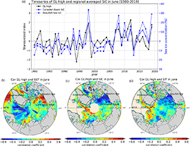
Figure 1. (a) Timeseries of June GL-high (black) and area-averaged SIC anomalies over the Canadian Basin (solid-blue line, reversed ordinate) and Beaufort Sea (dashed-blue line, reversed ordinate) from 1980 to 2019. The dashed-black line denotes the detrended timeseries of the GL-high. Stereographic plots of correlations between the June GL-high and (b) SST, (c) SIC and (d) SIT in June. Dots denote that the correlations greater than 0.32, exceeding the 95% confidence level. The Canadian-Basin and Beaufort-Sea SIC is defined as the area-averaged SIC over the domain: 114° W–150° W, 70° N–82° N and 114° W–150° W, 70° N–75° N, respectively.
Download figure:
Standard image High-resolution image3.2. Thermodynamic and mechanical redistribution processes
Firstly, the connection between the GL-high and the atmospheric circulation is examined. The regression maps between the June GL-high and H500, T850, Q850, 10 m wind divergence, OMEGA500 and LCC are shown in figure 2. Although the GL-high is defined by the H500 over Greenland, the positive geopotential anomalies extend further into the Central Arctic (figure 2(a)), consistent with [32]. Associated with an intensified GL-high, warm and moist air masses are advected to the west of Greenland from the northern Atlantic by southerly wind anomalies, resulting in a significant increase in temperature and humidity over the Baffin Bay, Baffin Island and Davis Strait (figures 2(b) and (c)). Due to the anomalously high geopotential over the Central Arctic, an intensified GL-high is associated with anomalously strong surface wind divergence around the Canadian Basin (figure 2(d)). According to the law of mass conservation, this leads to anomalous descending air motion, which is manifested as the significantly increased OMEGA500 over the Canadian Arctic Archipelago and Canadian Basin (figures 2(e) and (f)). The anomalous subsidence strengthens the climatological sinking motion, therefore there is less LCC (also total cloud cover, not shown) (figures 2(g) and (h)). This also contributes to the increased temperature over the Central Arctic and Canadian Arctic Archipelago due to the adiabatic heating (figure 2(b)). Associated with an intensified GL-high, the other reanalysis products (i.e. ERA5, NCEP2 and JRA55) also display increased descending air motion and decreased cloud cover around the Canadian Arctic Archipelago, suggesting that the circulation responses to variations in the GL-high are very robust (figure S2).

Figure 2. Regression maps between June GL-high and June (a) H500, (b) T850, (c) Q850, (d) 10 m wind divergence, (e) OMEGA500 and (g) LCC over the period 1980–2019. Figures (f) and (h) are the same as the (e) and (g) but for dataset of NARR. Stippling denotes that the regression coefficients exceed the 95% confidence level.
Download figure:
Standard image High-resolution imageSecondly, the CRF and surface radiative budget are displayed in figure 3. Clouds have a large influence on both incoming longwave (warming effect) and shortwave radiative (cooling effect) fluxes and therefore play a key role in the surface radiative balance [33–35]. As demonstrated in figure 3(a), due to the decreased LCC over the Canadian Basin (figures 2(g) and (h)), the CRF_SR is significantly increased with a magnitude of about 10 W m−2 (figure 3(a)). On the other hand, the CRF_LR is significantly reduced with a magnitude of about 5 W m−2 (figure 3(b)). Clearly, the CRF_SR is stronger than the CRF_LR, thus the total CRF is positive over the Canadian Basin. For surface radiative budget, an intensified GL-high is associated with a significant increase in downward shortwave radiation (DSR) over the Canadian Basin. Corresponding to one standard deviation increase of the GL-high, there is an increase in DSR of about 10 W m−2 for MERRA2 and about 15 W m−2 for APP-x and NARR (figures 3(c)–(e)). The increased DSR over the Beaufort Sea leads to sea ice melting by promoting ice–albedo feedback. In contrast, over the northeastern Canada and Davis Strait, the DSR is significantly decreased in the MERRA2, which is mainly due to the increased water vapor (figure 2(c)) that obstructs the incoming solar radiation [36]. A comparison between CRF_SR (figure 3(a)) and DSR (figure 3(c)) demonstrates that the increase of DSR in figure 3(c) is largely attributed to the reduced cloud cover, which substantially increases the CRF at the surface in figure 3(a). However, associated with the GL-high, there is little change in DLR over the Canadian Basin for MERRA2 and a significant decrease for APP-x and NARR (figures 3(f)–(h)), indicating that the DLR is not critical to the sea ice decline there. In terms of surface radiative balance, associated with one standard deviation increase of the GL-high, there is more than 15 W m−2 net radiative flux gain over the Beaufort Sea (figures 3(i)–(k)). Compared to the radiative fluxes, the surface turbulent heat fluxes are much smaller (not shown). This net gain of surface energy flux either warms up the surface air temperature, or is transmitted into the ocean, contributing to the bottom sea ice melting [37]. Previous studies have documented extensively the northward heat and moisture advection, and the enhanced DLR mechanism. Here, we shed light on the importance of the subsidence and reduced cloud cover, and the enhanced DSR mechanism on the sea ice loss over the Beaufort Sea, associated with variability of the GL-high. The importance of shortwave radiation for the summer Arctic sea ice has also been emphasized in several studies [38, 39], but not in relation to the GL-high.

Figure 3. Regression maps between June GL-high and June (a) CRF_SR (shortwave CRF), (b) CRF_LR (longwave CRF), (c) DSR, (f) DLR, and (i) NetRad at the surface over the period 1980–2019. Figures (d), (g), (j) and (e), (h), (k) are the same as the (c), (f), (i), but for datasets of APP-x and NARR, respectively. The corresponding datasets are labeled in brackets (i.e. MERRA2, APP-x and NARR). Stippling denotes that the regression coefficients exceed the 95% confidence level.
Download figure:
Standard image High-resolution imageFinally, we explore the mechanical redistribution of sea ice, which is closely related to the direction and strength of surface winds [5, 40]. Regression maps between zonal and meridional sea ice advection and the GL-high are shown in figures 4(a) and (b). Associated with an intensified GL-high, there is a significant anticyclonic wind anomaly over the Canadian Basin. Due to wind-driven sea ice motion, this is related to similar anomalously anticyclonic sea ice motion over the Arctic. For the zonal sea ice advection, an intensified GL-high is related to significant westward sea ice advection anomalies from the Canadian Basin to the Chukchi Sea. Note that over the Beaufort Sea both the wind speed and easterly wind frequency (percentage of days with easterly winds in June) are substantially increased (figures 4(c) and (d)). The strong easterly winds push sea ice away from the coast (e.g. Banks Island), leaving extensive open water areas [41–44]. This allows for greater absorption of DSR, leading to an increase in SST and thus a decrease in sea ice over the Beaufort Sea by promoting ice–albedo feedback. As for the meridional sea ice advection, an intensified GL-high is related to significant meridional advection of sea ice from the Chukchi Sea to the Svalbard Island via the Central Arctic (figure 4(b)). This corresponds to an intensified transpolar drift stream. Thus, there is a substantially increased SIC north of Svalbard and east of Greenland (figure 1(c)).

Figure 4. Regression coefficients between June GL-high and June (a) zonal area flux, (b) meridional area flux, (c) surface wind speed and (d) easterly wind frequency (percentage of days with easterly winds in June) (unit: %) over the period 1980–2019. The blue vectors in (a) denote the regression coefficients between the GL-high and surface winds, and in (b) denote the regression coefficients between the GL-high and sea ice motion. Stippling denotes that the regression coefficients exceed the 95% confidence level.
Download figure:
Standard image High-resolution imageFrom the above analysis, the mechanism behind the influence of an intensified GL-high on summer sea ice of the Beaufort Sea can be summarized as the combination of (a) thermodynamic process: increased subsidence around the Canadian Arctic Archipelago that results in reduced cloud cover and thus increased downward shortwave radiation, accelerating sea ice melt; and (b) dynamic process: increased anticyclonic anomalies around the Canadian Basin that drive the Beaufort-Sea ice away from the coast, promoting ice–albedo feedback.
3.3. Importance for seasonal Arctic sea ice prediction
The correlations between the GL-high and SIC, SST, SIT and Arctic SIE are displayed in figure 5. Similar to figures 1(b)–(d), statistically significant correlations between the GL-high in June and the SST, SIC, and SIT over the Canadian Basin are also found from July through September. During August and September, the sea ice over the northern Chukchi Sea is significantly correlated with the GL-high, which may be related to the modified transpolar drift stream in figure 4(b). The seasonal predictability of Beaufort-Sea SIC, SIT and SST arising from the GL-high can extend to November (figure 5, bar plot), indicating a strong coupling between the sea ice and oceanic processes [45]. In addition to the regional impacts, the June GL-high also impacts the seasonal evolution of the Arctic SIE with correlations around 0.50 in September and October (figure 5, purple bar), respectively. Note that the lagged correlations are much higher than the contemporaneous correlations. This is largely related to the enhanced meridional sea-ice advection (figure 4(b)) that spreads June sea-ice melting over the Beaufort Sea into the Central Arctic in the subsequent months. Overall, the results suggest that the GL-high in June is an important source of seasonal predictability for regional as well as total Arctic sea ice coverage.

Figure 5. Stereographic plots of correlations between the GL-high in June and Arctic SST, SIC and SIT from July through September. Dots denote that the correlations greater than 0.32, exceeding the 95% confidence level. Bar plot of correlations between the GL-high in June, and Beaufort-Sea SST (blue), Beaufort-Sea SIC (green), Beaufort-Sea SIT (red) and Arctic SIE (purple) from June through November. Note that the GL-high index is sign reversed for SIC, SIT and Arctic SIE. The black-dashed lines denote the correlation coefficients of 0.32, exceeding the 95% confidence level.
Download figure:
Standard image High-resolution image
4. Summary and discussion
This study investigates the impact of the GL-high in June on summer Arctic sea ice using atmospheric reanalysis datasets and satellite observations. We find that an intensified GL-high in June is associated with a significant decrease in sea ice over the Canadian Basin, particularly over the Beaufort Sea. The mechanism behind the influence is the combination of thermodynamic and mechanical redistribution processes. Firstly, an intensified GL-high is associated with significant wind divergence anomalies over the Canadian Basin, which leads to significantly increased subsidence there. As a result, there are fewer clouds, leading to significantly higher DSR over the Canadian Basin and Canadian Archipelago in MERRA2, APP-x and NARR. The increased DSR serves to accelerate sea ice decline over the Canadian Basin by amplifying ice–albedo feedback. Secondly, an intensified GL-high is also associated with strong offshore wind anomalies over the Beaufort Sea, pushing sea ice away from the coast and leading to larger open water areas. This also promotes ice–albedo feedback, contributing to substantial decrease in sea ice. This mechanism differs from previous findings, where moisture and heat advection and the accompanied increase in DLR are emphasized (e.g. [2]).
A case study for 2012 (see the supplementary material) also reveals the importance of the mechanism demonstrated in this study. In 2012, Arctic sea ice extent reaches a record low in the satellite era. Coincidently, the GL-high in June is the strongest (figure 1(a)) during our analysis period, which is associated with strong anticyclonic wind anomalies around the Canadian Arctic Archipelago (figure S6(a)). As a result, significant subsidence and decreased cloud cover anomalies are observed (figures S6(e) and (f)). This leads to a significant increase in DSR that further results in sea ice loss over the Beaufort Sea (figures S7(a) and (b)). We note that there is only a slight gain in DLR, indicating that DSR instead of the DLR accounts largely for the substantial sea ice decline over the Beaufort Sea in 2012 (figures S6(c) and (d)). Together with the intensified easterly winds (figure S8), the GL-high in June is responsible for the continuous sea ice decline and ocean warming in the following summer-to-fall months (figures S3–S5).
Although we emphasize the importance of the cloudiness-DSR mechanism, our results do not contradict the previous findings (e.g. [2]). As displayed in (2), the increased DLR associated with the anticyclonic anomalies over Greenland and the Arctic Ocean accounts for about 60% of the September Arctic SIE decline. This study added to previous findings by showing that the increased DSR and surface windspeed associated with an intensified GL-high contributes to about 20%–30% of the sea ice loss over the Beaufort Sea.
Acknowledgments
We thank three anonymous reviewers for their valuable and constructive comments. This work was supported by the National Key Research and Development Program of China (No. 2019YFC1509104) and (No. 2021YFC2802504), Innovation Group Project of Southern Marine Science and Engineering Guangdong Laboratory (Zhuhai) (No. 311021008).
Data availability statements
All the data analyzed here are openly available. The MERRA2 data are retrieved from the data portal at https://gmao.gsfc.nasa.gov/reanalysis/MERRA-2/. The APP-x data is obtained from https://nsidc.org/data/NSIDC-0669/versions/1. The NARR data are obtained from https://psl.noaa.gov/data/gridded/data.narr.html. The monthly sea ice concentration, sea ice motion, and sea ice extent are obtained from the NSIDC. The sea ice thickness is obtained from http://psc.apl.uw.edu/. The monthly SST is obtained from NOAA.
No new data were created or analyzed in this study.
Supplementary data (2.9 MB PDF)