


Abstract
Changes in spatial synchrony in the growing season have notable effects on species distribution, cross-trophic ecological interactions and ecosystem stability. These changes, driven by non-uniform climate change were observed on the regional scale. It is still unclear how spatial synchrony of the growing season on the climate gradient of the mid-high latitudes of the Northern Hemisphere and ecoregions, has changed over the past decades. Therefore, we calculated the start, end, and length of the thermal growing season (SOS, EOS, and LOS, respectively), which are indicators of the theoretical plant growth season, based on the daily-mean temperature of the Princeton Global Forcing dataset from 1948 to 2016. Spatial variations in the SOS, EOS and LOS along spatial climate gradients were analyzed using the multivariate-linear regression model. The changes of spatial synchrony in the SOS, EOS and LOS were analyzed using the segmented model. The results showed that in all ecoregions, spatially, areas with higher temperature tended to have an earlier SOS, later EOS and longer LOS. However, not all the areas with higher precipitation tended to have a later SOS, later EOS, and shorter LOS. The spatial synchrony in the SOS decreased across the entire study area, whereas the EOS showed the opposite trend. Among the seven ecoregions, spatial synchrony in the SOS in temperate broadleaf/mixed forests and temperate conifer forests changed the most noticeably, decreasing in both regions. Conversely, spatial synchrony in the EOS in the taiga, temperate grasslands/savannas/shrublands and tundra changed the most noticeably, increasing in each region. These may have important effects on the structure and function of ecosystems, especially on the changes in cross-trophic ecological interactions. Moreover, future climate change may change the spatial synchrony in the SOS and EOS further; however, the actual impact of such ongoing change is largely unknown.
Export citation and abstract BibTeX RIS

Original content from this work may be used under the terms of the Creative Commons Attribution 4.0 license. Any further distribution of this work must maintain attribution to the author(s) and the title of the work, journal citation and DOI.
1. Introduction
The plant growing season is the period of the year when plants grow and develop successfully, which regulates the exchange of carbon, water and energy between plants and the atmosphere (Piao et al 2008, Richardson et al 2013). Spatiotemporal variation in the growing season has an important influence on the structure and function of ecosystems (Vitasse et al 2018, Chen et al 2019, Piao et al 2019). Changes in spatial synchrony in the growing season are especially critical for the distribution of species, ecological interactions across trophic levels and ecosystem stability (Wang et al 2016, Pearson 2019, Rafferty et al 2020).
Approximately a hundred years ago, Hopkins (1920) proposed the bioclimatic law, which first quantified the geographical pattern of plant phenology in temperate North America. Driven by the recent climate change, temporal changes in the plant growing season have been observed on multiple scales (Jeong et al 2011, Ge et al 2015, Gill et al 2015). However, these changes varied among regions mainly due to the spatial non-uniform of climate change and differences in the sensitivity of the plant growing season to climate change (Menzel et al 2006, Vandvik et al 2018, Liu et al 2019). The spatial non-uniform in temporal changes of the plant growing season can cause changes of spatial synchrony. Several recent studies have also proved that the spatial synchrony in the growing season has already changed and these changes varied greatly among different regions (Wang et al 2015, 2016, Vitasse et al 2018, Liu et al 2019). Based on phenological observation data from 128 sites in the European Alps, Vitasse et al (2018) found that the altitude-induced shifts at the start of the growing season significantly decreased from 34 d km−1 in 1960 to 22 d km−1 in 2016. However, Cui et al (2018) analyzed the thermal growing season in northern China from 1961 to 2015 and found that the altitude-induced shifts at the start and end of the thermal growing season had increased and decreased, respectively. Wang et al (2015) examined the relationship between geographic location and temporal changes in the growing seasons in the USA and China, and found that the synchrony in the first bloom date between different latitudes had decreased. While Matsumoto (2010) examined the relationships between geographic location (latitude, longitude, and altitude) and temporal changes in budding and leaf fall dates in Japan, and found that only the synchrony in leaf fall date between different latitudes had decreased.
Until now, studies on the changes in spatial synchrony in growing season parameters have mainly been performed on a local or regional scale. Research on the mid-high latitudes of the Northern Hemisphere is very limited (Barichivich et al 2012, Liu et al 2019). Liu et al (2019) quantified changes in spatial synchrony in spring phenology from 1980–2009 to 2080–2099, and concluded that the spatial synchrony in spring phenology will increase under future warming conditions, due to the much greater spring warming at high latitudes, that even offset the effect of the lower temperature sensitivity of spring phenology at high latitudes. Barichivich et al (2012) analyzed the temporal changes in the thermal growing season from 1950 to 2011 and concluded that the lengthening of the thermal growing season was not uniform across the Northern Hemisphere, with stronger rates of extension in Eurasia than in North America. This implies that the spatial synchrony in the thermal growing season across the Northern Hemisphere has changed. Nevertheless, it is still not clear how spatial synchrony in the growing season changed in recent decades. Furthermore, current studies on changes in spatial synchrony in the growing season focus mainly on the relationships between the growing season and geographic location. However, climatic conditions are the determinant factors of plant growth and the biogeographical patterns of species (Rötzer and Chmielewski 2001, Xu et al 2018). Thus, it is necessary to estimate the spatial variation of the growing season along spatial climate gradients, that is, the spatial configuration relationship between the multiyear mean thermal growing season and climatic conditions. Additionally, the same ecoregion has common climatic characteristics, plant properties, and seasonal changes in plant growth, and similar responses to management practices (Olson et al 2001, Zhou et al 2003, Hargrove et al 2009). Studies have shown that the growing season and its changes varied among ecoregions (Zhu et al 2012, Ji et al 2021). Therefore, we also calculated the variations in the growing season along spatial climate gradients, and changes in spatial synchrony in the thermal growing season at the ecoregion scale.
We calculated the thermal growing season, based on the daily mean temperature, which theoretically refers to the period when it is warm enough for plant growth. Studies have shown that the warming rates were not uniform across the mid-high latitudes of the Northern Hemisphere and the warming was faster at higher latitudes than at lower latitudes, implying that the spatial difference in temperature was reduced (Serreze et al 2009, Cohen et al 2014; which can also be seen in the figures S1 and S2 (available online at stacks.iop.org/ERL/16/124017/mmedia)). Thus, we specifically addressed two hypotheses: (a) Spatial synchrony in the thermal growing season across the mid-high latitudes of the Northern Hemisphere had increased. (b) Changes in spatial synchrony in the thermal growing season varied among ecoregions. Consequently, the main aims of this study were: (a) to quantitatively analyze variations in the thermal growing season along spatial climate gradients in the mid-high latitudes of the Northern Hemisphere and in each ecoregion, and (b) to explore how the spatial synchrony in the thermal growing season changed in the mid-high latitudes of the Northern Hemisphere and in each ecoregion.
2. Materials and methods
2.1. Ecoregions
We followed the ecoregion classification from the World Wildlife Fund in The Global 200: Priority Ecoregions for Global Conservation (figure 1, https://geospatial.tnc.org/) (Wiken 1986, Bailey 1995, Olson and Dinerstein 2002). The main reason for choosing the mid-high latitudes of the Northern Hemisphere is due to the obvious seasonal variation of vegetation in these locations (Wang et al 2019). Because the growing season of plants in the Mediterranean is mainly limited by available water, the definition of the thermal growing season is not applicable; therefore Mediterranean forests/woodlands/scrub were excluded (Kramer et al 2000, Peñuelas et al 2002).
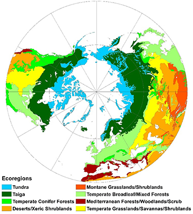
Figure 1. Spatial distribution of ecoregions in the study area (Wiken 1986, Bailey 1995, Olson and Dinerstein 2002). Reproduced with permission from Olson and Dinerstein (2002).
Download figure:
Standard image High-resolution image2.2. Climatic data
We obtained the daily mean temperature and precipitation data for 1948–2016 with a spatial resolution of 0.25° from the Princeton Global Forcing dataset (PGF, http://hydrology.princeton.edu/data.pgf.php). The daily mean temperature data were used to estimate the parameters of the thermal growing season. We calculated the multiyear mean annual temperature and the multiyear mean annual precipitation (MAT and MAP) based on the daily mean temperature and precipitation. The PGF dataset was constructed by combining a suite of observation-based datasets with the National Centers for Environmental Prediction/National Center for Atmospheric Research reanalysis dataset (Sheffield et al 2006).
2.3. Methods
2.3.1. Definition of the thermal growing season
The thermal growing season is the period of year when it is theoretically warm enough for plant growth, and is generally defined as the period when the daily mean temperature continuously exceeds a certain threshold (Carter 1998, Cui et al 2018). Compared to the growing season estimated by remote sensing datasets (1980s–present, the highest temporal resolution is 5 d), the thermal growing season has a longer time-series (1950s–present) and higher temporal resolution (daily). This study adopted the definition of the thermal growing season used by Peterson et al (2001), in which its start (SOS) is considered the last day of the first 5 d spell with a daily mean temperature above 5 °C, and its end (EOS) is considered the first day of the first 5 d spell with a daily mean temperature below 5 °C. The length of the thermal growing season (LOS) is the number of days between the SOS and EOS.
2.3.2. Statistical analyses
Spatial variations in the mean SOS, EOS and LOS along spatial climate gradients were determined based on multivariate linear regression models:

where  is the mean SOS, EOS, and LOS for 1948–2016 for a pixel.
  are the multiyear mean annual temperature and precipitation of the corresponding pixels, respectively.
  is the intercept,
  are regression coefficients, and
  is the residual.
Since the 1980s, the Northern Hemisphere has experienced sustained and rapid warming, which may be the hottest period in the past 1400 years (Stocker 2014, Morice et al 2021). To compare the difference between the thermal growing season before and after the rapid warming, we divided the period of 1948–2016 into two sub-periods: 1948–1981 and 1982–2016. Using 1982 as the cut-off makes the degrees of freedom of the two sub-periods equal.
The trends in the SOS, EOS and LOS for 1948–1981, 1982–2016, and 1948–2016 were calculated as the slope of the linear regression using ordinary least squares:
where  is the SOS, EOS, and LOS of a pixel in a given year,
  is the intercept,
  is the slope,
  is the year, and
  is the residual.
We applied the nonparametric Wilcoxon matched-pairs signed ranks test to detect whether the distributions of the trend and mean SOS, EOS, and LOS from 1948–1981 to 1982–2016 changed.
The coefficient of variation (CV) is an index that can effectively reflect the degree of variation of numerical variables. The CV is the ratio of the standard deviation to the mean and is usually expressed as a percentage. It has no dimension and can eliminate the influence of numerical units and mean values when comparing the degree of variation among multiple variables. Therefore, the CV can be used to study the degree of spatial variation of the mean SOS, EOS, and LOS for 1948–1981 and 1982–2016. The greater the CV, the greater the degree of variation around the mean, meaning, the wider the data's distribution range (Whelen and Siqueira 2018, Tang et al 2021).
The segmented model was applied to estimate the relationships between the mean SOS, EOS, and LOS for 1948–1981 and their changes from 1948–1981 to 1982–2016. The segmented model estimates the broken line relationship comprising the breakpoints and slope parameters of the linear relationship changes, which is an improvement of the linear regression (Bausch 2008).
ArcGIS 10.4 (ESRI 2016) was used to produce geospatial distribution maps. All statistical analyses and data visualizations were performed in R-studio (Team 2016) using R version 3.5.1 (Team 2018), and the raster (Hijmans 2016), ncdf4 (Pierce and Pierce 2019), ggpubr (Kassambara and Kassambara 2020), and segmented (Muggeo and Muggeo 2017) packages.
3. Results
3.1. Spatial distribution of the mean SOS, EOS, and LOS for 1948–2016
As expected, in the mid-high latitudes of the Northern Hemisphere, there were large spatial differences in the SOS, EOS, and LOS (figure 2). The mean SOS in the mid-latitudes occurred earlier, mainly before day of year (DOY) 135 (15 May), where those in the high latitudes and Tibetan Plateau occurred later, mainly after DOY 150 (1 June). Contrastingly, the mean EOS occurred later in the mid-latitudes, mainly after DOY 285 (12 October), while those in the high-latitudes and Tibetan Plateau occurred earlier, mainly before DOY 270 (27 September). The mean LOS ranged from 17 d at higher latitudes to 310 d at lower latitudes.

Figure 2. Spatial distributions (a)–(c) and frequency distributions (d) of the mean start, end, and length of the thermal growing season (SOS, EOS, and LOS, respectively) for 1948–2016. Gray areas represent areas without an obvious detectable annual cycle in the thermal growing season.
Download figure:
Standard image High-resolution imageAcross the mid-high latitudes of the Northern Hemisphere, the spatial distributions of the SOS, EOS and LOS were significantly consistent with the spatial distributions of the multi-year MAT and MAP (table 1). Spatially, areas with higher temperature tended to have earlier SOS, later EOS, and longer LOS. The mean SOS, EOS and LOS were advanced by 4.0 d, delayed by 3.1 d and extended by 7.1 d, respectively, for every 1 °C increase in MAT. Spatially, areas with higher precipitation tended to have later SOS, later EOS, and shorter LOS. The mean SOS, EOS and LOS were delayed by 1.3 d, delayed by 0.3 d and shorted 1.0 by days, respectively, for every 100 mm increase in MAP.
Table 1. Spatial regression analyses between climatic conditions and the mean start, end, and length of the thermal growing season (SOS, EOS, LOS, respectively) for 1948–2016.
| Parameters | β_MAT (days/°C) | β_MAP (days/100 mm) | R2 |
|---|---|---|---|
| SOS | −4.0 | 1.3 | 0.85 |
| EOS | 3.1 | 0.3 | 0.87 |
| LOS | 7.1 | −1.0 | 0.88 |
MAT and MAP are the multi-year mean annual temperature and precipitation, respectively.
3.2. Temporal changes in the SOS, EOS, and LOS
3.2.1. Spatial distribution of the overall trends
There were also large spatial differences in the SOS, EOS, and LOS trends during 1948–2016 (figure 3). For the SOS, 39% of evaluated pixels showed significant negative trends. The pixels with an advanced SOS were mainly distributed in central and northern Asia, central Europe, and western and central North America. Approximately 22% of the pixels showed significant positive trends toward a later EOS, which were mainly distributed in central and northern Asia, northeastern Europe, and northern North America. Only 0.6% of the pixels showed significantly negative trends toward an earlier EOS, which were sparsely distributed in central Europe and northwestern North America. Almost half the pixels showed significant trends toward a longer LOS, which were mainly distributed in central and northern Asia, central and western Europe, and western and northern North America.

Figure 3. The spatial distributions of trends in the start, end, and length of the thermal growing season (SOS (a) and (b), EOS (c) and (d), and LOS (e) and (f), respectively) during 1948–2016. p < 0.05 indicates that the trend was significant at the 0.05 level. Gray areas represent areas without an obviously detectable annual cycle in the thermal growing season or areas without a significant trend.
Download figure:
Standard image High-resolution image3.2.2. Differences in the SOS, EOS, and LOS between 1948–1981 and 1982–2016
The trend distributions in the SOS, EOS, and LOS were significantly different between 1948–1981 and 1982–2016 (Wilcoxon matched-pairs signed ranks test, p < 0.05; figures 4, S3 and S4). During 1948–1981, almost half the evaluated pixels showed negative trends toward an earlier SOS. During 1982–2016, approximately 66% of the pixels showed negative trends toward an earlier SOS. Compared to the SOS, the differences in the trends of the EOS and LOS between the two periods were larger. Approximately 63% of the pixels showed negative trends toward an earlier EOS during 1948–1981; however, almost 85% showed positive trends toward a later EOS during 1982–2016. Similarly, the percentage of pixels showing positive trends toward a longer LOS changed from 44% during 1948–1981 to 85% during 1982–2016. Generally, trends in the advanced SOS, delayed EOS, and extended LOS, during 1982–2016, were steeper than those during 1948–1981.
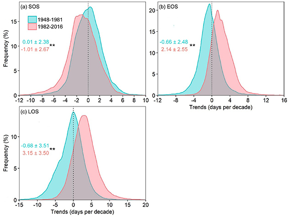
Figure 4. Differences in the trend distributions at the start, end, and length of the thermal growing season (SOS (a), EOS (b), LOS (c), respectively) between 1948–1981 and 1982–2016. Numbers in cyan and coral colors represent means ± standard deviations for 1948–1981 and 1982–2016, respectively. ** indicate differences at p < 0.05 using the nonparametric Wilcoxon matched-pairs signed ranks test. The black vertical straight dotted lines indicate that the trends of the thermal growing season were 0.
Download figure:
Standard image High-resolution imageDistributions of the mean SOS, EOS, and LOS for 1948–1981 and 1982–2016 were significantly different (Wilcoxon matched-pairs signed ranks test, p < 0.001; figure 5). Compared to1948–1981, the mean SOS, EOS, and LOS for 1982–2016 had advanced by 4.0 ± 3.4 d (mean ± standard deviation), delayed by 2.5 ± 3.5 d, and extended by 6.5 ± 4.6 d, respectively. The CV of the mean SOS increased from 24.01% during 1948–1981 to 25.73% during 1982–2016, indicating that the SOS timing became more spatially variable. Contrastingly, the CV of the mean EOS decreased from 9.72% during 1948–1981 to 9.27% during 1982–2016, indicating that the EOS timing became less spatially variable. The CV of the mean LOS decreased from 40.41% during 1948–1981 to 38.79% during 1982–2016, indicating that the EOS timing became less spatially variable.
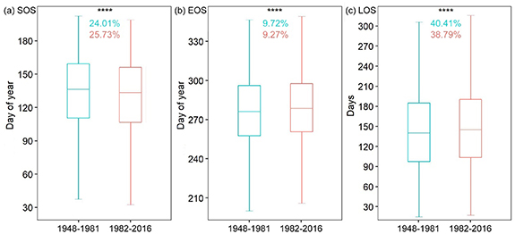
Figure 5. Differences in the distributions of mean start, end, and length of the thermal growing season (SOS (a), EOS (b), and LOS (c), respectively) between 1948–1981 and 1982–2016. Numbers in cyan and coral colors represent CVs for the periods of 1948–1981 and 1982–2016, respectively. **** indicates differences at p < 0.001 using the nonparametric Wilcoxon matched-pairs signed ranks test.
Download figure:
Standard image High-resolution imageChanges in the mean SOS, EOS, and LOS from 1948–1981 to 1982–2016 were inconsistent across the mid-high latitudes of the Northern Hemisphere (figure 6). When the mean SOS for 1948–1981 was less than 136, it was significantly positively correlated with its change for 1982–2016. This indicates that pixels with an earlier SOS from 1948 to 1981 exhibited further advances than other pixels in the SOS from 1982 to 2016. However, when the mean SOS for 1948–1981 was greater than 136, there was no relation with its change for 1982–2016. The EOS means for 1948–1981 before and after the breakpoint, both significantly negatively correlated with their changes for 1982–2016. This indicates that pixels with an earlier EOS from 1948 to 1981 exhibited further delays than other pixels in the EOS from 1982 to 2016. When the mean LOS for 1948–1981 was less than 123 d, it significantly negatively correlated with its change for 1982–2016, indicating that pixels with a shorter LOS from 1948 to 1981 exhibited further extensions than other pixels in the LOS from 1982 to 2016. However, when the mean LOS for 1948–1981 was larger than 123 d, it significantly positively correlated with its change for 1982–2016, indicating that pixels with an longer LOS from 1948 to 1981 exhibited further extensions than other pixels in the LOS from 1982 to 2016.

Figure 6. Relationship between the mean start, end, and length of the thermal growing season (SOS (a), EOS (b), and LOS (c), respectively) for 1948–1981 and its change for 1982–2016. Straight red dotted lines indicate that the differences of the mean SOS, EOS, and LOS between the two periods were 0. Straight solid lines are the fitting segmented regression lines, and the blue and red lines are the fitting lines before and after breakpoints, respectively. The breakpoints in a–c are 136, 265, and 123, respectively.
Download figure:
Standard image High-resolution image3.3. Variations in the SOS, EOS, and LOS across different ecoregions
3.3.1. Variations in the SOS, EOS, and LOS along the spatial climate gradients
In each ecoregion, the spatial distributions of the mean SOS, EOS and LOS were significantly consistent with spatial distributions of MAT and MAP (table 2). Among them, consistency was highest in the temperate grasslands/savannas/shrublands (TGSS) and lowest in the tundra. In all ecoregions, areas with higher temperature tended to have an earlier SOS, later EOS, and longer LOS. In the montane grasslands/shrublands (MGS), the mean SOS, EOS, and LOS advanced by 6.1 d, delayed by 5.2 d and extended by 11.3 d for every 1 °C increase in the MAT, respectively, which were the largest changes among the seven ecoregions. In the tundra, the mean SOS, EOS and LOS were only advanced by 1.0 d, delayed by 1.9 d and extended by 2.9 d for every 1 °C increase in the MAT, respectively.
Table 2. Spatial regression analyses between climatic conditions and the start, end, and length of the thermal growing season (SOS, EOS, LOS, respectively) for 1948–2016 in different ecoregions.
| Parameters | TBMF | TGSS | Taiga | Tundra | TCF | DXS | MGS | |
|---|---|---|---|---|---|---|---|---|
| SOS | β_MAT (days/°C) | −5.5 | −4.1 | −2.8 | −1.0 | −4.7 | −4.6 | −6.1 |
| β_MAP (days/100 mm) | 0.9 | −0.1 | 2.2 | −0.5 | 0.8 | −0.7 | 1.1 | |
| R2 | 0.79 | 0.93 | 0.69 | 0.24 | 0.73 | 0.87 | 0.84 | |
| EOS | β_MAT (days/°C) | 3.7 | 3.3 | 2.2 | 1.9 | 4.0 | 3.4 | 5.2 |
| β_MAP (days/100 mm) | 1.2 | 0.9 | 0.8 | 0.6 | −0.3 | 1.9 | 0.6 | |
| R2 | 0.87 | 0.95 | 0.79 | 0.47 | 0.80 | 0.94 | 0.84 | |
| LOS | β_MAT (days/°C) | 9.2 | 7.4 | 5.0 | 2.9 | 8.7 | 8.0 | 11.3 |
| β_MAP (days/100 mm) | 0.3 | 1.0 | −1.5 | 1.1 | −1.1 | 2.6 | −0.5 | |
| R2 | 0.88 | 0.96 | 0.78 | 0.42 | 0.79 | 0.92 | 0.87 | |
MAT and MAP represent the multiyear mean annual temperature and precipitation, respectively. DXS, MGS, TBMF, TCF and TGSS are the deserts/xeric shrublands, montane grasslands/shrublands, temperate broadleaf/mixed forests, temperate conifer forests, and temperate grasslands/savannas/shrublands, respectively.
In contrast to the MAT, relationships between MAP and the mean SOS, EOS, and LOS were inconsistent among ecoregions. In the TGSS, tundra and DXS (deserts/xeric shrublands), areas with higher precipitation tended to have an earlier SOS, contrary to what was seen in the other four ecoregions. For every 100 mm change in MAP, the mean SOS changed by 2.2 d in taiga and 0.1 d in TGSS, which was the largest and smallest change, respectively, among the seven ecoregions. Areas with higher precipitation tended to have an earlier EOS only in the temperate conifer forests (TCF), contrary to what was seen in the other ecoregions. For every 100 mm change in MAP, the mean EOS had the largest and the smallest change in DXS (1.9 d) and TCF (0.3 d), respectively. In the MGS, TCF, and taiga, areas with higher precipitation tended to have a shorter LOS, contrary to what was seen in the other ecoregions. For every 100 mm change in MAP, the mean LOS had the largest and smallest change in DXS (2.6 d) and temperate broadleaf/mixed forests (TBMF) (0.3 d), respectively. The relationships between MAP and the mean SOS, EOS, and LOS were greatly affected by the spatial configurations of precipitation and temperature, which are usually controlled by atmospheric circulation characteristics and weather systems.
3.3.2. Temporal changes in the SOS, EOS, and LOS of different ecoregions
The mean SOS, EOS, and LOS for 1982–2016 were significantly earlier, later, and longer than those for 1948–1981 in all ecoregions (Wilcoxon matched-pairs signed ranks test, p < 0.001; figure 7). Among the seven ecoregions, the longest and shortest advances in the SOS were observed in TBMF (6.1 ± 4.8 d) and tundra (2.9 ± 2.2 d), respectively. However, the longest and shortest delays in the EOS were observed in tundra (4.8 ± 3.9 d) and TBMF (0.8 ± 3.4 d), respectively. The longest and shortest extensions in the LOS were observed in tundra (7.7 ± 4.8 d) and MGS (4.5 ± 6.1 d), respectively. From 1948–1981 to 1982–2016, the SOS timing in all ecoregions became more spatially variable (table 3). The change in the CV of the mean SOS was greatest in TBMF, increasing from 20.88% during 1948–1981 to 24.63% during 1982–2016. The EOS timing in MGS and TBMF became more spatially variable, in contrast to what was seen in the other ecoregions. The change in the CV of the mean EOS was greatest in tundra, increasing from 6.22% during 1948–1981 to 5.73% during 1982–2016. Additionally, only the LOS in TBMF became more spatially variable. The change in the CV of the mean LOS was greatest in the tundra, decreasing from 33.70% during 1948–1981 to 29.25% during 1982–2016.
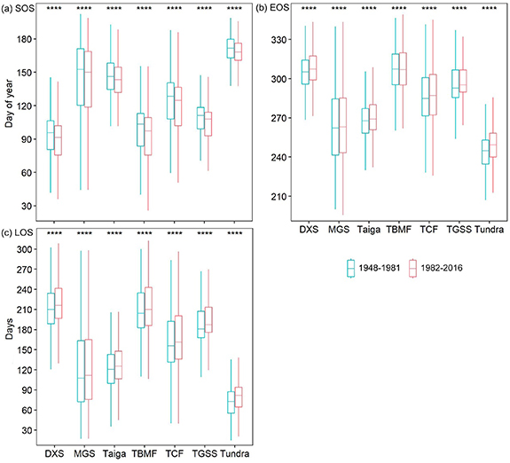
Figure 7. Distributions of mean start, end, and length of the thermal growing season (SOS (a), EOS (b), and LOS (c), respectively) for 1948–1981 and 1982–2016 in different ecoregions. **** indicates differences at p < 0.001 using the nonparametric Wilcoxon matched-pairs signed ranks test. DXS, MGS, TBMF, TCF, and TGSS are the deserts/xeric shrublands, montane grasslands/shrublands, temperate broadleaf/mixed forests, temperate conifer forests, and temperate grasslands/savannas/shrublands, respectively.
Download figure:
Standard image High-resolution imageTable 3. The CVs of the start, end, and length of the thermal growing season (SOS, EOS, and LOS, respectively) for 1948–1981 and 1982–2016 in different ecoregions.
| Ecoregions | DXS | MGS | Taiga | TBMF | TCF | TGSS | Tundra | |
|---|---|---|---|---|---|---|---|---|
| SOS | 1948–1981 | 21.89% | 22.47% | 10.42% | 20.88% | 20.31% | 16.47% | 6.87% |
| 1982–2016 | 22.81% | 23.43% | 10.77% | 24.63% | 22.51% | 18.25% | 6.90% | |
| Percentage increase | 4.20% | 4.27% | 3.36% | 17.96% | 10.83% | 10.81% | 0.44% | |
| EOS | 1948–1981 | 4.69% | 10.87% | 5.66% | 4.76% | 7.55% | 5.27% | 6.22% |
| 1982–2016 | 4.66% | 10.91% | 5.36% | 4.85% | 7.27% | 4.95% | 5.73% | |
| Percentage increase | −0.64% | 0.37% | −5.30% | 1.89% | −3.71% | −6.07% | −7.88% | |
| LOS | 1948–1981 | 16.37% | 50.82% | 23.98% | 16.04% | 28.18% | 17.58% | 33.70% |
| 1982–2016 | 15.74% | 49.64% | 22.48% | 16.55% | 27.71% | 17.04% | 29.25% | |
| Percentage increase | −3.85% | −2.32% | −6.26% | 3.18% | −1.67% | −3.07% | −13.20% |
DXS, MGS, TBMF, TCF, and TGSS are the deserts/xeric shrublands, montane grasslands/shrublands, temperate broadleaf/mixed forests, temperate conifer forests, and temperate grasslands/savannas/shrublands, respectively.
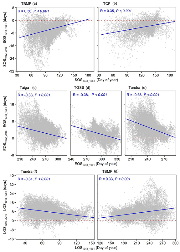
Among the ecoregions, the correlation between the SOS and its changes was stronger in TBMF and TCF, where pixels with an earlier SOS exhibited a more advanced SOS than that of other pixels (figures 8(a) and (b)). The correlation between the EOS and its changes was stronger in the taiga, TGSS, and tundra (figures 8(c)–(e)), where pixels with an earlier EOS exhibited a more delayed EOS than that of other pixels. The correlation between the LOS and its changes was stronger in the tundra and TBMF (figures 8(f) and (g)), where pixels with a shorter LOS exhibited a more and less extended LOS than that of other pixels in the tundra and TBMF, respectively.
Figure 8. Relationship between the mean start, end, and length of the thermal growing season (SOS (a) and (b), EOS (c)–(e), and LOS (f) and (g), respectively) from 1948 to 1981 and changes from 1982–2016 in the ecoregions. Notably, only the ecoregions with a correlation coefficient greater than 0.3 are shown here. The details of the other ecoregions can be seen in figures S5–S7. TBMF, TCF, and TGSS are the temperate broadleaf/mixed forests, temperate conifer forests, and temperate grasslands/savannas/shrublands, respectively. Straight red dotted lines indicate that the differences in the mean SOS, EOS, and LOS between the two periods was 0. Straight blue solid lines are linear regression lines.
Download figure:
Standard image High-resolution image
4. Discussion
4.1. Changes in the thermal growing season
We found that from 1948 to 2016, the SOS, EOS, and LOS were advanced, delayed and extended, respectively. However, the most change occurred in the second half of the study period (1982–2016), which coincided with accelerated warming during this period (Shen et al 2012, Barichivich et al 2013, Zhu et al 2019). Similarly to our results, Barichivich et al (2012) reported that the LOS had extended substantially in the mid-high latitudes of the Northern Hemisphere during 1950–2011, but most of the extension occurred during 1980–2011. Similarly, Dong et al (2012) found that during 1980–2009, the SOS advance, EOS delay, and LOS extension in the Tibetan Plateau were steeper than those during 1960–1979.
Importantly, we also found that in the entire study area, pixels with an earlier SOS and EOS exhibited a more advanced SOS and delayed EOS. This provides evidence that the spatial synchrony in the SOS has decreased, whereas the EOS shows the opposite, which is not completely consistent with our first hypothesis. Arctic amplification has been observed in spring, autumn and winter and has been the greatest in autumn (Serreze et al 2009, Hansen et al 2010, Screen and Simmonds 2010, Cohen et al 2014). This implies that the spatial distributions of temporal changes in the SOS and EOS do not always match the spatial distributions of the seasonal temperature changes. From the analysis of the temporal and spatial variations of the warming rates, we found that the warming rates not only varied across space, but also varied within a year, which was greatest in spring and least in summer (figures S1 and S2). From the definition of the SOS/EOS used here, the SOS/EOS depends more on the temperature in a small window of the year. Therefore, we calculated temporal change trends of the mean temperature during the SOS/EOS occurrence period from 1948 to 2016 (figure S8). The results showed that the warming rates in the pixels where the SOS/EOS occurred earlier were greater than those in the pixels where the SOS/EOS occurred later, which is consistent with the spatial distribution of the temporal changes of the SOS and EOS. Therefore, we surmise that the main reason for the spatial mismatch between the temporal change of the SOS and spring temperature change might be that the SOS of the evaluated pixels did not focus on spring, but varied greatly across space, from early-spring to mid-summer (12 March–27 June). However, the EOS of the evaluated pixels mainly occurred in the autumn (23 August–18 November), which might be the main reason for the spatial match between the temporal change of the EOS and autumn temperature change. Moreover, the seasonal temperature changes can be interpreted as the temperature variation within the same time window of a year, whereas the temporal changes of the SOS and EOS can be interpreted as the variation of the time reaching a certain temperature threshold in a year. Therefore, the variation in the SOS (EOS) was related to but not identical to the spring (autumn) temperature change.
Additionally, the extension was steeper at the short and long LOS than at the intermediate LOS, implying that the spatial distributions of temporal changes in the LOS did not match the spatial distributions of the annual mean temperature changes. This might be related to potentially different degrees of warming in different seasons, such as more or less snow (precipitation-related); thus, earlier or later spring onset can occur due to climate warming.
4.2. Ecological implications of changes in the thermal growing season
Changes in the thermal growing season may affect multiple ecological levels, from the individual to the ecosystem. For example, the frost risk of buds may increase with advancement of the SOS (Inouye 2008, Augspurger 2013, Kim et al 2014). Because most flowering plants rely on animals for pollination (Cohen et al 2014), and climate change does not necessarily cause identical changes in anthesis and pollinators (Schweiger et al 2008), there might be a mismatch between them. Thus, TBMFs with the longest SOS advancement might face the greatest frost risk, and mismatch between anthesis and pollinators, among the seven ecoregions. EOS delays tend to produce larger increases in ecosystem respiration than photosynthesis (Randerson et al 1999, Piao et al 2008). They might also increase carbon uptake, which is most likely to occur in tundra, which have the longest EOS delays. Because the distribution limits of plants are defined by marginal climatic conditions, the alleviation of climatic constraints may promote their northern/southern migration (Morin et al 2007, Boisvert-Marsh 2012). LOS extensions in a given ecotone may provide suitable conditions for the settlement of southern plants (Taggart and Cross 2009, Boisvert-Marsh 2012). Tundra having the longest LOS extensions are more likely to be invaded by plants from adjacent southern ecoregions, evidenced by reports on the northward migration of taiga into tundra (Yansa 2006, Boisvert-Marsh et al 2014).
Consistent with the second hypothesis, changes in spatial synchrony in the thermal growing season varied among different ecoregions. This may alter the interactions and dynamics of populations and affect individual survival, species adaptability, and ecosystem stability (Dai et al 2014, Wang et al 2016, Prevéy et al 2017, Vitasse et al 2018). Among ecoregions, spatial synchrony of the SOS changed most noticeably in TBMFs and TCFs, decreasing in both regions. This implies that the overlap in anthesis over space might have decreased, resulting in decreased pollen flow (gene flow) and greater reproductive isolation (Bonner 2017, Rafferty et al 2020). Gosper et al (2005) reported that many migrants, such as birds, primarily consume fruits during autumn migration, which many plants rely on to disperse their seeds. The spatial synchrony of the EOS changed most noticeably in taiga, TGSSs, and tundra, increasing in each region. This might create mismatch between migrant arrival and fruit ripening in wintering and stopover habitats, resulting in decreased seed dispersal (Gill et al 2015). More detailed studies are required to evaluate the ecological effects of changes in spatial synchrony in the thermal growing season.
The results of this study were based on the PGF dataset, chosen mainly because of its high spatial resolution and long time period. Changes in the source of the dataset will likely not change the main conclusions. On the one hand, many forcing datasets have the same inputs (Yin et al 2018), such as, the inputs of CRU-NCEP and PGF that include both NCEP and CRU datasets (Sheffield et al 2006, Lawrence et al 2019). On the other hand, all forcing datasets are bias-corrected based on the CRU time-series (Müller et al 2016). According to Müller et al (2016), the spatial and temporal variations of temperature across the Northern Hemisphere are very similar among five state-of-the-art climate forcing datasets. Although the magnitude of the annual total precipitation obtained from different forcing datasets is highly inconsistent, especially in areas with sparse field observations, all datasets capture similar spatial precipitation patterns over the Northern Hemisphere (Gehne et al 2016, Sun et al 2018). Therefore, although there are discrepancies between different forcing datasets, changes in the source of datasets may not affect this study's main conclusions.
Furthermore, because many climate forcing factors often operate at fine spatial resolutions (microclimate), our research using a coarse-resolution climate forcing dataset may obscure the thermal growing season's intra-pixel heterogeneity (Lembrechts et al 2020). Microclimatic heterogeneity can buffer species against the impacts of climatic changes (Ohlemüller et al 2008, Suggitt et al 2018). Therefore, microclimatic heterogeneity could also buffer against the impact of changes in the thermal growing season. Further studies using multiple spatial data (from fine to coarse spatial scales) to more accurately study the changes in the thermal growing season, and the effects of these impacts, are required.
5. Conclusions
In 1948–2016, the spatial variation of the thermal growing season was consistent with the spatial variation of the climatic conditions in the mid-high latitudes of the Northern Hemisphere, and in each ecoregion. Among these seven ecoregions, spatially, areas with higher temperature tended to have an earlier SOS, later EOS, and longer LOS, whereas not all the areas with higher precipitation tended to have a later SOS, later EOS, and shorter LOS. The spatial synchrony of the SOS and EOS on the climate gradient changed in the entire study area and in each ecoregion. The spatial synchrony of the SOS in the TBMFs and TCFs changed most noticeably, decreasing in both regions. The EOS spatial synchrony in taiga, TGSSs, and tundra changed most noticeably, increasing in each region. Changes in the spatial synchrony of the thermal growing season on the climate gradient may profoundly affect species distribution, cross-trophic ecological interactions, and ecosystem stability. More attention should be paid to the potential consequences of these phenomena.
Acknowledgments
The work presented here was carried out in collaboration between all authors. F W and Y J conceived and designed the work; F W, Y J, Y W and S Z analyzed and interpreted the data; F W and Y J drafted the manuscript; F W, Y J, Y W, S Z and H X revised the manuscript.
Data availability statement
The data that support the findings of this study are openly available.
No new data were created or analysed in this study.
Funding
This work was supported by the National Key Research and Development Program of China (Grant Number 2018YFA0606101) and the National Natural Science Foundation of China (Grant Numbers 41630750 and 42171049).
Conflict of interest
The authors declare that they have no conflict of interest exists.