


Abstract
Climate warming has been driving hydrological changes across the globe, especially in high latitude and altitude regions. Long-term (1962–2012) streamflow records and permafrost data in the Yangtze River source region were selected to analyze streamflow variations and groundwater storage in response to climate warming. Results of Mann–Kendall test and Morlet wavelet analysis show that the anomalies of both annual streamflow and winter baseflow are near the year 2010, and their main period scales are 37 years and 34 years, respectively. The annual streamflow and the annual baseflow increased significantly, as assessed by the recursive digital filtering baseflow separation. Results of Pearson correlation coefficient indicate that the rising air temperature is the primary cause for the increased streamflow instead of precipitation and evaporation. By using the top temperature of permafrost model, the total permafrost area has decreased by 8200 km2 during the past 50 years, which causes groundwater storage to increase by about 1.62 km3 per year due to climate warming. More space has been made available to store the increasing meltwater during the permafrost thawing. Permafrost thawing and increasing temperature are the direct and indirect causes of the increasing groundwater storage. The results of the cumulative anomaly method and Pearson correlation coefficients show that permafrost thawing has a greater impact than increasing temperature on the increase of groundwater storage. Permafrost thawing due to climate warming show compound effects on groundwater storage–discharge mechanism, and significantly affects the mechanisms of streamflow generation and variation.
Export citation and abstract BibTeX RIS

Original content from this work may be used under the terms of the Creative Commons Attribution 4.0 license. Any further distribution of this work must maintain attribution to the author(s) and the title of the work, journal citation and DOI.
1. Introduction
Climate warming on the Qinghai–Tibet Plateau (QTP) is more significant than any other regions around the world (Held and Soden 2006). Previous studies show that the warming rate on the QTP is higher than those of the global average, and its temperature is expected to be even higher in the future decades (Kang et al 2007, Kuang and Jiao 2016). One of the direct effects of climate warming is the degradation of permafrost in the QTP (Cheng and Wu 2007, Yang et al 2010, Feng et al 2019). Over the past four decades, the permafrost area in the QTP has decreased from 1.50 × 10⁶ km2 to 1.26 × 10⁶ km2 (Cheng and Jin 2013, Cheng et al 2019). Wu et al (2012) revealed that the thickness of the active layer (the soil layer above the permafrost that freezes in winter and thaws in summer) on the QTP experienced a significant increase at a rate of 6.3 cm yr−1 between 2006 and 2010, and the trend of active layer thickening was basically consistent with the increasing trend of annual average temperature (Xu et al 2017).
The three rivers' source region, which contains the Mekong River, the Yangtze River, and the Yellow River, is located in the QTP. The geological and hydrological conditions of the QTP are critical to water conservation and ecological security of China (Mahmood et al 2020). Streamflow in the Yangtze River source region has undergone great changes in response to climate warming. Several studies analyzed the periodicity of streamflow and climatic factors and concluded that the streamflow increased significantly and it was highly related to climatic factors (Li 2018, Xu et al 2019, Ahmed et al 2020). The annual streamflow in the Yangtze River source region is increasing prominently and there are significantly positive correlations among streamflow, precipitation, and temperature, and a significantly negative correlation between streamflow and water surface evaporation (Luo et al 2019). Qian (2013) calculated the baseflow of the Yangtze River source region and the contribution rate of various climatic factors (precipitation, temperature and evaporation) and permafrost to the streamflow. The previous studies focused on analyzing streamflow from the perspective of periodicity, and the influences of climatic factors and permafrost on streamflow variations. However, the relationship between streamflow and groundwater storage changes triggered by permafrost thawing were not included.
The existence of permafrost limits the infiltration and migration of groundwater. The hydrologic process and groundwater circulation in the permafrost area are greatly restricted (Rowland et al 2010). Permafrost thawing causes the groundwater circulation channels to be deeper and longer and the increase of underground water volume, which will affect the exchange between surface water and groundwater (Chang et al 2008, Walvoord and Kurylyk 2016). Shi et al (2015) divided the spring runoff into five typical values (the 5 percentile, 10 percentile, 50 percentile, 90 percentile, and 95 percentile of spring runoff, respectively), and then analyzed the relationship among the five typical flow values, hydrologic factors, and climatic factors by the Mann–Kendall non-parameter test method. Lyon et al (2009), Lyon and Destouni (2010) linked the degradation of frozen soil with the regression coefficient and found that the regression coefficient could be used to characterize the degradation of frozen soil.
Previous studies have shown that due to the warming climate and the degradation of permafrost, the thickness of the active layer in the permafrost region increases, and the groundwater will be released with the deepening of the active layer, i.e. it may lead to the increase of groundwater storage (Walvoord and Striegl 2007, Zarnetske et al 2008, Jacques and Sauchyn 2009, Muskett and Romanovsky 2009). Ge et al (2011) concluded that the thickening of the active layer can increase groundwater discharge. Many studies also proved that the increase of winter baseflow and annual mean streamflow in permafrost regions is mainly related to the increase of groundwater storage caused by permafrost thawing (Painter 2011, Duan et al 2017, Lamontagne et al 2018, Xu et al 2018). These studies linked the permafrost thawing with groundwater storage. However, they concentrated on permafrost and lacked in deeper analysis of the variations of groundwater storage. Many studies concluded that the terrestrial water storage (total vertically integrated water storage including groundwater storage, soil moisture storage, and snow water equivalent storage) and groundwater storage in the QTP were increased by using the gravity recovery and climate experiment (GRACE) satellite data (Wang et al 2020, Chao et al 2020). However, the GRACE data started from 2002 and were too short to analyze the groundwater storage changes. Lin et al (2020) quantitatively estimated the groundwater storage according to the baseflow recession in winter in the upper Lhasa River, which could fill the blank in the incomplete GRACE data. Liu et al (2020) found that there is a mutual consistency between changes derived from GRACE data and the baseflow recession in the central Yangtze River basin. Recognizing the groundwater storage, especially its periodicity characteristics, is important to predict the recharge and discharge of the groundwater under climate warming. However, to the best of our knowledge, there is no study on the periodicity of groundwater storage and quantitative assessment of the impact of permafrost thawing on groundwater storage in the Yangtze River source region.
In this study, we aim to quantify the impacts of permafrost thawing on streamflow and groundwater storage in the Yangtze River source region under climate warming. The aims of this study are: (a) to analyze the characteristics of streamflow and its influencing factors; (b) to analyze the trends of groundwater storage and its periodicity characteristics; (c) to estimate the relationship between groundwater storage and permafrost thawing.
2. Materials and methods
2.1. Study area
The area of the Yangtze River source region is about 13.77 × 10⁴ km2, which is located in the central QTP (figure 1). It is one of the most representative alpine areas in China with the most concentrated biodiversity and it has undergone significant changes due to climate warming (Jiang et al 2015, Grosse et al 2016, Wang et al 2017). The main rivers in the region are the Tuotuo River, Dangqu River and Chumar River. The downstream of the Tuotuo River is referred to as the Tongtian River, which is the largest trunk stream and its change could affect the streamflow in the whole source region (Chorography Compile Committee of Qinghai Province 2000). The climate in the source region is a continental and transitional type, which is mainly controlled by the upper Westerly belt (Cao 2013). The mean annual air temperature ranges from −5.5 °C to −1.7 °C, the annual mean precipitation is 375.4 mm, and the annual evaporation is between 1340 mm and 1700 mm (Li et al 2020).

Figure 1. (a) Location of the Yangtze River source region in China. (b) Location of the hydrological station at Zhimenda, four meteorological stations at Wudaoliang, Qumalai, Yushu, and Tuotuohe, and four main rivers including the Chumar River, Tuotuo River, Tongtian River, and Dangqu River in the study area.
Download figure:
Standard image High-resolution image2.2. Data
Streamflow data were obtained from the most upstream hydrological station of the Yangtze River (Zhimenda Station). Temperature, precipitation, and evapotranspiration were obtained from the four meteorological stations in Tuotuohe, Wandaoliang, Qumalai, and Yushu (table 1, http://data.cma.cn). Weighted average of the meteorological data were calculated by the Thiessen polygon (Thiessen 1911, Bhavani 2013, Panno and Luman 2018). Permafrost data were simulated by the top temperature of permafrost (TTOP) model (
Table 1. Basic information of the meteorological stations in the Yangtze River source region.
| Station | Latitude (°N) | Longitude (°E) | Elevation (m) | Area (×104 km2) |
|---|---|---|---|---|
| Wudaoliang | 35.22 | 93.08 | 4612.2 | 2.59 |
| Tuotuohe | 34.22 | 92.43 | 4533.1 | 6.67 |
| Qumalai | 34.13 | 95.78 | 4175.0 | 3.93 |
| Yushu | 33.02 | 97.03 | 3681.2 | 0.67 |
2.3. Methods
2.3.1. Trend analysis and mutation detection
Time series is often analyzed as a whole for its statistical characteristics. They often exhibit abrupt changes under the compound effects of other factors in the dynamical system, namely mutation, and the mutation points indicate specific years after which the time series shows this kind of abrupt changes (Mann 1945). Hydrological time series are affected by climate and human activities, and they have undergone significant changes, therefore, the primary step of trend analysis and investigating the impact of environmental changes on hydrological processes is to find out the mutation points (Burn and Hag 2002). Cumulative anomaly and Mann–Kendall test are the most common methods to determine the trend and mutation of time series because they have simpler evolution characteristics and more obvious trends than other methods in trend detecting (Mann 1945, Renner and Bernhofer 2011, Wang et al 2011).
2.3.1.1. Cumulative anomaly method
Cumulative anomaly method (
2.3.1.2. Mann–Kendall test
Mann–Kendall test ( and
and  (
( is the forward sequence which can be calculated as equation (A16),
  is the backward sequence which is calculated as equation (A17), the intersection of the two curves indicates a mutation point (Mann 1945, Sneyers 1975, Pirnia et al
2019). If
is the backward sequence which is calculated as equation (A17), the intersection of the two curves indicates a mutation point (Mann 1945, Sneyers 1975, Pirnia et al
2019). If  in equation (A16) is more than the significance levels such as α = 0.2 (α is the significance level,
  ), it represents low confidence level. Similarly, α = 0.1 (
 ) represents moderate confidence level, and α = 0.05 (
 ) represents high confidence level (Bao et al
2012, Güçlü 2020).
) represents high confidence level (Bao et al
2012, Güçlü 2020).
2.3.2. Wavelet analysis
Wavelet analysis is a frequently used method in trend analysis of time series. Wavelet analysis can identify the periodicity of time series and investigate temporal patterns from both frequency and time domains (Labat et al 2004, Adamowski and Sun 2010). Contour maps of the real part of wavelet coefficients and wavelet variograms can intuitively represent the main period of time series (Labat et al 2005, Kang et al 2007). The Morlet continuous complex wavelet transform was used to analyze the variations of streamflow in the Yangtze River source region (Morlet et al 1982, Staszewski 1998, Nakken 1999, Sang et al 2013, Michael 2019). Table 2 shows the similarities and differences between wavelet analysis and the mutation detection methods.
Table 2. Similarities and differences between wavelet analysis and mutation detection methods.
| Cumulative anomaly method | Mann–Kendall test | Wavelet analysis | |
|---|---|---|---|
| Introduction | A basic method in analyzing trend characteristics and determining mutation points of different time series. | The most widely used and effective method in detecting trends of hydrological and meteorological series, which is of higher accuracy than other methods. | The most common method in identifying the periodicity of hydrological and meteorological time series. |
| Differences | Aiming at trend analysis in the past years. | Aiming at trend prediction in the near future. | |
| Similarities | All of them are aiming at analyzing the statistical characteristics of different time series. | ||
2.3.3. Baseflow separation
The recursive digital filtering method is one of the most reliable methods for separating baseflow due to its high accuracy, since it eliminates the random interference and proves the detection accuracy (Bozic 1976, Eckhardt 2005, Stamenković et al 2019):
where  is the daily baseflow (m3 d−1) subject to
  <
<  ,
,  is the time step (day),
  is the daily discharge (m3 d−1),
  is a dimensionless recession constant and
  ,
,  is the maximum value of the ratio of baseflow to total streamflow with
  . The
. The  is tightly related to the total baseflow, and
  controls the shape of baseflow hydrograph.
2.3.4. Estimation of groundwater storage
Groundwater storage is estimated by three main functions (Brutsaert and Nieber 1977, Malvicini et al 2005):

where  is the volumetric flow rate in winter baseflow (m3 d−1),
  is the total amount of groundwater storage in the catchment aquifers (m3),
  and
and  are the dimensionless constants depending on the hydrogeological conditions of the study area.
  is the baseflow recession coefficient, which is a parameter that could quantitatively represent the streamflow recession process of the catchment.
  is a parameter that typically ranges from 0.5 to1.0.
During the dry season, when there is no precipitation and other inputs, the conservation of mass equation can be expressed as follows (Brutsaert and Nieber 1977, Parlange et al 2001, Brutsaert 2008, Lin et al 2020):
Substitution of equation (2) into equation (3) leads to (Brutsaert and Nieber 1977, Mendoza et al 2003, Rupp et al 2004, Rupp and Selker 2006):
where  is the temporal change in the baseflow during recession, and constants
  and
and  are the intercept and slope of the plots of
  versus
  in log–log space. Parameters of
  and
and  in equation (2) can be expressed in terms of
  and
and  as
as ![$K = 1{\textrm{ }}/\left[ {a\left( {2 - b} \right)} \right]$](https://content.cld.iop.org/journals/1748-9326/16/8/084011/revision3/erlac0f27ieqn35.gif) and
and  (Lyon et al
2009, Gao et al
2017).
(Lyon et al
2009, Gao et al
2017).
3. Results
3.1. Assessment of streamflow variation
Figure 2 shows the 5% (Q5%), 10% (Q10%), 25% (Q25%), 50% (Q50%), 75% (Q75%), and 90% (Q90%) dates of the annual total streamflow between 1962 and 2012. For example, the 5 percentile date (Q5%) is the day by which the 1st 5% of the annual streamflow has occurred in the catchment. The 10% (Q10%), 25% (Q25%), 50% (Q5%), 75% (Q75%), and 90% (Q90%) dates are defined in the same way. The Q50% date is similar to the 'date of center of mass of flow' (Stewart et al 2005, Hodgkins and Dudley 2006). According to these data, we can infer the relationship between streamflow and seasons. The occurrence time of the six typical annual streamflow (Q5%, Q10%, Q25%, Q50%, Q75% and Q90%) in the Yangtze River source region shows a significantly upward tendency except Q25% and Q50% from 1961 to 2012 (figure 2). The slopes of the dates of Q5%, Q10%, Q75%, and Q90% are increasing mean the dates of these four typical flows are delayed. Delaying dates indicates there are much more precipitation first becoming groundwater and then discharging into river instead of discharging into the river directly. The slopes of the dates of Q25% and Q50% are decreasing mean the dates of these two typical flows are advanced. The advance in dates is mainly caused by the melt of the solid water remaining in winter and the dates are advanced by rising temperature. The dates of Q25% and Q50% are in summer (from June to August) according to the results, so we estimate that the variations of streamflow are closely related to seasons.

Figure 2. Variations of the occurrence time of 5% (Q5%), 10% (Q10%), 25% (Q25%), 50% (Q50%), 75% (Q75%), and 90% (Q90%) of the annual streamflow between 1962 and 2012, respectively.
Download figure:
Standard image High-resolution imageIn order to determine the mechanisms of the streamflow variation, we first chose the recursive digital filtering method to separate baseflow from the streamflow. Figure 3 shows that the increasing trends of the streamflow and baseflow are close to each other, with the slopes of 1.68 m3 s−1 and 1.35 m3 s−1 per year, respectively, indicating that the increase of baseflow plays an important role in the increase of streamflow.  in the graph ranges from 0.68 to 0.74, which means the annual mean
  is relatively stable.
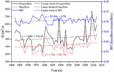
Figure 3. Variations in the annual streamflow, baseflow,  (the ratio of baseflow to the total streamflow) and their linear trends between 1962 and 2012.
Download figure:
Standard image High-resolution imageThe Mann–Kendall test shows that annual streamflow and winter baseflow exhibit a significantly increasing trend at the 95% confidence level ( = 0.05) during 1962–2012 (figure 4). The values of
  show the variation of corresponding time series,
  represents the decrease of time series, and the larger the absolute value of
  is, the greater the decrease is. Figure 4 shows that there is a significant decrease of both streamflow and baseflow near the year 1966, and a shortly increase since 2010. The annual streamflow decreases more sharply in 1972–1981 and 1996–2000 (
 = 0.05), while the winter baseflow is in 1979–1981 (
 = 0.05). The intersection at the beginning is not representative, and it has been often ignored in the Mann–Kendall test (Li et al
2011). Therefore, annual streamflow's mutation point of 1965 is removed and the mutation years of the annual streamflow are 2008 and 2011 (figure 4). The mutation year of winter baseflow is 2008, which is the same as the result of previous studies (Li et al
2017).
= 0.05). The intersection at the beginning is not representative, and it has been often ignored in the Mann–Kendall test (Li et al
2011). Therefore, annual streamflow's mutation point of 1965 is removed and the mutation years of the annual streamflow are 2008 and 2011 (figure 4). The mutation year of winter baseflow is 2008, which is the same as the result of previous studies (Li et al
2017).
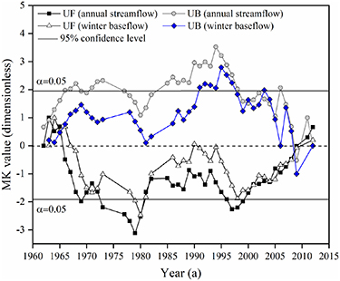
Figure 4. Detection of Mann–Kendall mutation points of the annual streamflow and winter baseflow. ( and
and  are two important dimensionless parameters in the Mann–Kendall test according to equations (A12)–(A17), the intersections of them with a 95% confidence level (
 = 0.05) of the time series represent the mutation points, indicating specific years after which the time series shows abrupt changes.)
Download figure:
Standard image High-resolution image3.2. Assessment of wavelet analysis
The contour map of the real part of wavelet coefficients depicts the periodic characteristics of streamflow time series in different time scales. When the real part of the wavelet coefficients is positive, it represents wet year, and negative represents dry year. The vertical coordinates corresponding to the centers of contour lines represents the main period scales and the horizontal coordinates represents the wet years or dry years. The characteristics of wetness–dryness alternation at main period scales are helpful to predict streamflow variations in the next period scales. Figure 5(a) shows that the 1st main period scale is 37 a for streamflow variation. There are three wet years (1966, 1989, and 2008) and two dry years (1976 and 1998) of the annual streamflow in the 37 a, which means it has five obvious wetness–dryness alternations (first increases and then decreases) at the period scale of 37 a.
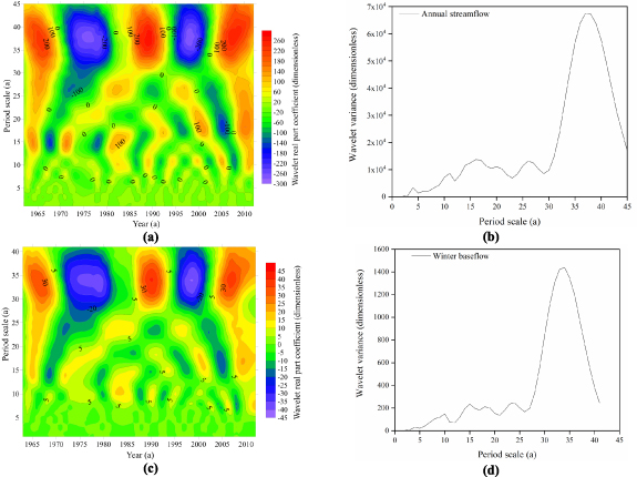
Figure 5. Temporal fluctuations and corresponding Morlet wavelet analysis of the annual streamflow and winter baseflow during 1962–2012 (unit 'a' in the parentheses means year). (a) The contour map of the real part of annual streamflow; (b) the wavelet variogram of annual streamflow; (c) the contour map of the real part of winter baseflow; (d) the wavelet variogram of winter baseflow.
Download figure:
Standard image High-resolution imageThe wavelet variogram can reflect the distribution of fluctuation energy and determine the main period precisely in different time series, and it has been widely used in analyzing streamflow variations. There are five obvious peaks in figure 5(b), corresponding to the time scales of 11 a, 20 a, 26 a, 16 a, and 37 a from small to large. The maximum peak is 37 a, indicating that the period scale of 37 a is the strongest, and 37 a is the 1st main period of the streamflow variation. That is to say, there is a 37 years periodicity (five obvious wetness–dryness alternation at the period scale of 37 a) in streamflow variation, which is consistent to the results in figure 5(a). The periodic fluctuation energy of the remaining time scales of 16 a, 26 a, 20 a, and 11 a decreases successively. Time scales of 37 a, 16 a, 26 a, 20 a, and 11 a are the 1st to 5th main periods of annual streamflow. The above five periods control the characteristics of streamflow variations during 1962–2012.
Similarly, the winter baseflow wavelet variogram indicates that the winter baseflow also have five significant periods, from the 1st to the 5th main periods are 34 a, 15 a, 24 a, 18 a, and 10 a, respectively (figure 5(c)). The periodic oscillation energy in 34 a is the largest, controlling the variation in the winter baseflow (figure 5(d)). Continuous hydrologic years should be chosen during the wavelet analysis of winter baseflow. As there are no streamflow data in 1974–1976, 1983–1984, and 2010, winter baseflow cannot be calculated in 1962, 1977, 1985, and 2011. The winter baseflow's period scales are smaller than those of the annual streamflow. But the five main period scales of both winter baseflow (34 a, 15 a, 24 a, 18 a, and 10 a) and annual streamflow (37 a, 16 a, 26 a, 20 a, and 11 a) are similar. According to the obvious wetness–dryness alternations (first increase and then decrease) of streamflow and baseflow in their 1st main periods, both the streamflow and baseflow are possibly increasing significantly in the near future.
3.3. Estimation of groundwater storage by baseflow recession
Daily baseflow records in winter (December–February) were used in calculating the groundwater storage. Figure 6(a) shows all data points of  versus
  in log–log space during 1962–2012. The fitted slope
  of the blue dashed line is equal to 1.02 via the nonlinear least squares fit from equation (4). It should be noted that the value of real intercept is its corresponding log value in figure 6(a), it is
  according to equation (4). The values of
  and
and  then can be calculated as 42.25 and 0.98, respectively. The total amount of the groundwater storage
  for each year can be directly estimated by equation (2). Figure 6(b) compares the groundwater storage estimated by baseflow recession analysis during 1962–2012 and the terrestrial water storage estimated by reconstructing GRACE data (Li et al
2021) during 1990–2012. The height difference between two curves mainly includes the soil moisture storage and snow water equivalent storage. The two curves in figure 6(b) are well correlated with a Pearson's correlation coefficient (Pearson 1895, Fischer et al
2017) of 0.63 during 1990–2012, which is higher than the previous study (Liu et al
2020). The coefficient indicates a generally good correlation between the baseflow-derived groundwater storage and the GRACE-derived measurements. As groundwater storage is essentially directly derived from streamflow data, there are some uncertainties in the estimated groundwater storage. One of the main uncertainties is from neglecting glacier melt water. Human activities and vegetation were also not taken into account.
for each year can be directly estimated by equation (2). Figure 6(b) compares the groundwater storage estimated by baseflow recession analysis during 1962–2012 and the terrestrial water storage estimated by reconstructing GRACE data (Li et al
2021) during 1990–2012. The height difference between two curves mainly includes the soil moisture storage and snow water equivalent storage. The two curves in figure 6(b) are well correlated with a Pearson's correlation coefficient (Pearson 1895, Fischer et al
2017) of 0.63 during 1990–2012, which is higher than the previous study (Liu et al
2020). The coefficient indicates a generally good correlation between the baseflow-derived groundwater storage and the GRACE-derived measurements. As groundwater storage is essentially directly derived from streamflow data, there are some uncertainties in the estimated groundwater storage. One of the main uncertainties is from neglecting glacier melt water. Human activities and vegetation were also not taken into account.
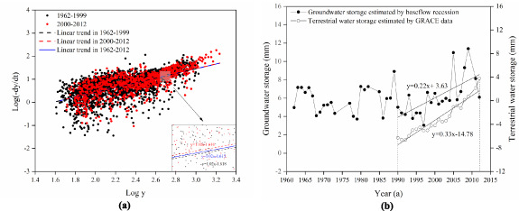
Figure 6. (a) Data points of  versus y as well as the linear recession curve in log–log space in three periods (1962–1999, 2000–2012, and 1962–2012) by using baseflow recession analysis. (b) Variations in groundwater storage estimated by baseflow recession analysis during 1962–2012 and terrestrial water storage estimated by reconstructing GRACE data (Li et al
2021) during 1990–2012.
versus y as well as the linear recession curve in log–log space in three periods (1962–1999, 2000–2012, and 1962–2012) by using baseflow recession analysis. (b) Variations in groundwater storage estimated by baseflow recession analysis during 1962–2012 and terrestrial water storage estimated by reconstructing GRACE data (Li et al
2021) during 1990–2012.
Download figure:
Standard image High-resolution imageFigure 7 depicts the variations in three kinds of parameters (slope  , intercept
  , and coefficient
  ) in equation (4) of all the recession data points (from December to February), they are processed by moving average according to the 1st to 5th main periods of streamflow (sliding windows at 37 a, 16 a, 26 a, 20 a, and 11 a, respectively). Figure 7 shows that the variations in these three parameters (slope
  , intercept
  , and coefficient
  ) are related to the five main periods of the annual streamflow. The stronger the periodicity is, the larger the absolute values of slopes in three pictures are (figures 7(a)–(c)). This indicates there is a positive correlation between the increase of groundwater recession coefficient
  in equation (4) and the 1st to 5th main periods of the streamflow in the Yangtze River source region from 1962 to 2012. As shown in figure 7(a), the variations of slope
  of the fitted recession curves in equation (4) during each period gradually move upward, which are opposite to the results of the intercept's variation (figure 7(b)). As the slope
  increases, the intercept
  gradually decreases, and the recession coefficient
  increases (figure 7(c)). Furthermore, the three figures are at a confidence level of 95% (α = 0.05), and this long-term variation in the recession coefficient
  from December to February indicates that baseflow recession gradually speeds up in the catchment during winter.
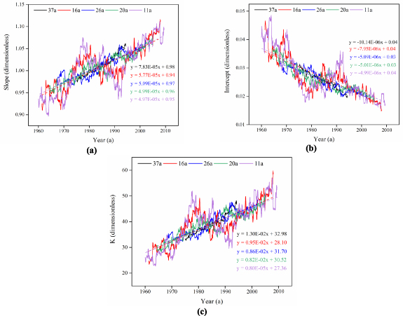
Figure 7. Variations in (a) the slope b; (b) the intercept a; (c) the recession coefficient  in equation (4) as well as their linear trends processed by moving average according to the 1st to 5th main periods of streamflow (sliding windows at 37 a, 16 a, 26 a, 20 a, and 11 a, respectively).
Download figure:
Standard image High-resolution image4. Discussion
4.1. Analysis of streamflow variations
Analyzing variation of streamflow and its influencing factors in the Yangtze River source region is vital to the variation of water resources in the middle and lower reaches of the Yangtze River and the entire QTP. Streamflow and baseflow show decreasing trends during 1960–1979, while  shows an increasing trend. The streamflow and baseflow reached a minimum in 1979 (figure 3). The streamflow and baseflow fluctuate significantly after 1980. The reason is that the annual mean precipitation in the region increased rapidly in the 1980s, 1990s, and 21st century (Wu et al
2020). So the period from 1980 to 2012 was selected as the period for focused analysis.
shows an increasing trend. The streamflow and baseflow reached a minimum in 1979 (figure 3). The streamflow and baseflow fluctuate significantly after 1980. The reason is that the annual mean precipitation in the region increased rapidly in the 1980s, 1990s, and 21st century (Wu et al
2020). So the period from 1980 to 2012 was selected as the period for focused analysis.
The streamflow in the source region is correlated with climatic factors including temperature, precipitation, and evapotranspiration. In order to investigate the periodic characteristics and multi-year variation of the climatic factors, daily data from meteorological stations of Tuotuo River, Wudaoliang, Qumalai, and Yushu between 1962 and 2012 (table 1) were analyzed according to the Thiessen polygon method. The wavelet periodic analysis and the Mann–Kendall test were also used to investigate the variation characteristics of the various climatic factors (table 3). The result of Morlet wavelet analysis shows the 1st to 6th periods of the annual mean temperature are 26 a, 36 a, 16 a, 8 a, 11 a, and 5 a, respectively (figures 8(a) and (b)). The 26 a period is the most significant period scale that can reflect the variation characteristics during 1962–2012. According to the obvious wetness–dryness alternations (first increase and then decrease) of temperature in figure 8(a), we predict that the annual mean temperature would be a rising tendency in the near future (Michael 2019). The periods of the annual mean precipitation are 37 a, 26 a, 20 a, 17 a, 7 a, and 10 a, respectively (figures 8(c) and (d)), which shows a similar increasing trend as temperature. For evapotranspiration, the periods are 36 a, 26 a, 21 a, 17 a, and 6 a, respectively (figures 8(e) and (f)). The wavelet variogram of evapotranspiration implies that it will also be increasing in the following years.
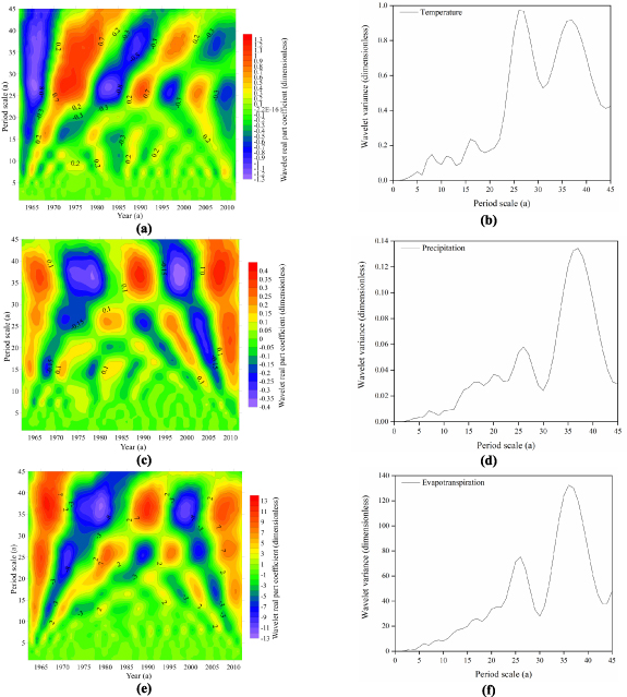
Figure 8. Temporal fluctuations and corresponding Morlet wavelet analysis of the climatic factors available in the Yangtze River source region during 1962–2012 (unit 'a' in the parentheses means year): the contour maps of the real part of (a) temperature; (c) precipitation; (e) evapotranspiration; and the wavelet variograms of (b) temperature; (d) precipitation; (f) evapotranspiration.
Download figure:
Standard image High-resolution imageTable 3. The period scales and mutation points of each climatic factors and streamflow.
| Elements | Period scales (a) | The 1st main period (a) | Mutation points |
|---|---|---|---|
| Temperature | 26, 36, 16, 8, 11, 5 | 26 | 1998 |
| Precipitation | 37, 26, 20,17, 7, 10 | 37 | 2005 |
| Evapotranspiration | 36, 26, 21, 17, 6 | 36 | 1982, 1989, 2002 |
| Streamflow | 37, 16, 26, 20, 11 | 37 | 2008, 2011 |
On the basis of the Pearson correlation coefficient between the three climatic factors and streamflow, the correlation from high to low is annual average temperature (0.68) > rainfall (0.43) > evapotranspiration (0.34). Such correlations suggesting that the increase of streamflow in the Yangtze River source region during 1962–2012, especially after 1980, is closely related to climate warming.
4.2. Relation between groundwater storage and permafrost thawing
Permafrost thawing under climate warming can significantly influence the mechanism of streamflow (Walvoord and Kurylyk 2016). A reasonable hypothesis is that increased groundwater storage in winter is highly related to permafrost thawing, and the permafrost thawing may enlarge the groundwater storage capacity (Lyon and Destouni 2010, Niu et al
2016). The TTOP model has been validated to be of high adaptability in simulating the permafrost areal extent and distribution in the Yangtze River source region (Smith and Riseborough 1996, Nan 2003, Reich et al
2017). The results show that the permafrost area in the catchment has undergone great changes. Figure 9 clearly shows the degradation of permafrost from 1962 to 2012. The distribution of seasonally frozen soil or no permafrost area in 1962 is mainly concentrated in the southeast of the study area, and then extended to the northwest area along the river net in 2012. The permafrost area decreased from 13.39 × 10⁴ km2 (97% of the study area) in 1962 to 12.57 × 10⁴ km2 (91% of the study area) in 2012, which has decreased by 8200 km2 (figure 10). The minimum permafrost area of 9.69 × 10⁴ km2 (70% of the study area) occurs in 2006. There is a significant downward trend after 1995. Figure 10 shows the annual mean permafrost area is decreasing at a rate of 401 km2 a−1 during 1962–2012, and total groundwater storage  shows an increase trend at a rate of 1.62 km3 a−1. Since the variations of the permafrost area and
  are highly relative to streamflow and streamflow has a significant downward trend after 1980, we choose the typical period of 1980–2012 for a detailed analysis.

Figure 9. Permafrost area and distribution simulated by the TTOP model in (a) 1962; (b) 2012.
Download figure:
Standard image High-resolution image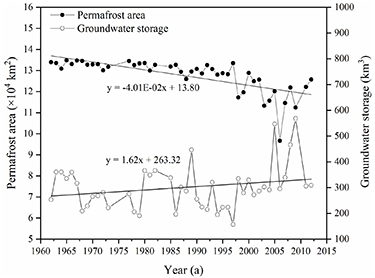
Figure 10. Variations in permafrost area, groundwater storage and their linear trends during 1962–2012.
Download figure:
Standard image High-resolution imageFigure 11 shows that the annual mean permafrost area decreased at 577 km2 a−1 between 1980 and 2012. In order to eliminate the effect of extreme values, all the data in figure 11 were processed by moving average (a sliding window at 10 years) based on the data in 1980–2012 from figure 10. The variation of permafrost area during 1997–2012 is much more fluctuant than that of 1980–1997. As shown by the cumulative anomaly curves (figure 12), the anomaly of permafrost area is 1997, so we divided the trend analysis into two sections before and after 1997. The annual mean permafrost area decreasing rates are −334 km2 a−1 in 1980–1997 and −425 km2 a−1 in 1997–2012, respectively (figure 11). The fluctuation in 1997–2012 is comparatively larger than that in 1980–1997 and its slope is closer to the overall trend, revealing that the variation of permafrost area is mainly influenced by the period after 1997. The year of 1997 is close to the mutation point of annual mean temperature (1998), indicating that the variation of permafrost area is closely related to the variation of temperature. Meanwhile, the permafrost area shows an increasing trend and the groundwater storage shows a decreasing trend after 2008 (figure 11).
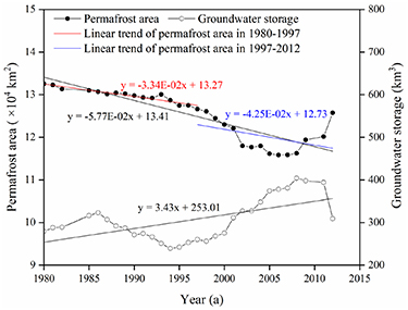
Figure 11. Variations of permafrost area, groundwater storage and their linear trends after moving average (a sliding window at 10 years) for the typical period of 1980–2012.
Download figure:
Standard image High-resolution image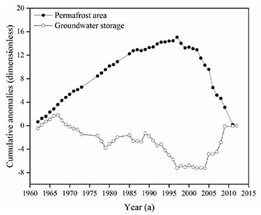
Figure 12. Cumulative anomaly curves of permafrost area and groundwater storage.
Download figure:
Standard image High-resolution image
The groundwater storage increases from 279 km3 in 1980 to 309 km3 in 2012 and its increasing rate is 3.43 km3 a−1 in this period (figure 11). The cumulative anomaly of groundwater storage is 2004 as shown in figure 12. The weighted average of the mutations of all the time series can be calculated out is 2000 (table 4). So we divided groundwater storage into two periods (before and after 2000) for a better understanding of its trends (figure 6(a)). The blue solid line in figure 6(a) depicts the fitted linear trend of  in 1962–2012, with a slope of 1.02. The linear trends in 1962–1999 (the black dash line) and 2000–2012 (the red dash line) are also shown in figure 6(a). The change of intercept
  due to slope
  in equation (4) can be observed to be an increasing trend from 0.0241 in 1962–1999 to 0.0245 in 2000–2012. The result means the absolute values of both the coefficient
  and the groundwater storage are increasing about 1.8% after 2000.
Table 4. The mutations of all data by using the Mann–Kendall test and the cumulative anomaly method.
| Elements | Mann–Kendall test | Cumulative anomaly method |
|---|---|---|
| Temperature | 1998* | 1996 |
| Precipitation | 2005* | 1997 |
| Evapotranspiration | False | 1982*, 1989*, 2002* |
| Streamflow | 2008*, 2011* | 2004 |
| Baseflow | 2008* | 2004 |
| Permafrost area | False | 1997* |
| Groundwater storage | 2006* | 2004 |
Note: False in the table means the results of the Mann–Kendall test is out of range, and the mutation point is determined by cumulative anomaly method. * in the table means the final mutation point.
The correlation coefficients between groundwater storage and permafrost area and between groundwater storage and temperature in 1980–2012 can be calculated to be 0.74 and 0.67 by the Pearson correlation coefficient method. The correlation coefficients indicate that they are negatively correlated, and the variation of groundwater storage is more closely correlated with the permafrost area than temperature. Therefore, melt water in the permafrost is released as permafrost thaws, influencing the variation of water resources in the whole Yangtze River source region. The groundwater storage in the near future is predicted to be increasing according to the periodicity analysis of the baseflow, as baseflow first increases and then decreases in its 1st main period (figure 5).
5. Conclusions
In this study, changes in hydrological and climatic elements were analyzed in order to identify the main climatic factor of streamflow changes in the Yangtze River source region. The Morlet wavelet analysis of the periods of temperature, precipitation, evapotranspiration, streamflow, and baseflow shows that both precipitation and streamflow have the main periods of 37 a, the main periods of evapotranspiration (36 a) and baseflow (34 a) are also close to the period of 37 a. The annual streamflow, especially the baseflow, increases significantly during 1962–2012, and the rising air temperature acts as the primary factor for the increased streamflow instead of precipitation and evapotranspiration.
The total permafrost area has decreased by 8200 km2 from 1962 to 2012 under a warming climate. The alternation of streamflow mechanism due to permafrost thawing increased the capacity of groundwater storage, and triggered a significant increase in groundwater storage at a rate of approximately 1.62 km3 a−1. There is a positive correlation between the increase of groundwater recession coefficient  in equation (4) and the main periods of the streamflow (37 a, 16 a, 26 a, 20 a and 11 a). The recession gradually speeds up in the Yangtze River source region from 1962 to 2012. There is a negative correlation between groundwater storage and permafrost area. The increase of groundwater storage in 1962–2012, especially after 1980, is closely related to the permafrost thawing. The findings are of great significance to the study of future hydrological processes and water resources management in the QTP and other similar alpine regions in the world.
Acknowledgments
We thank the anonymous reviewers for their helpful comments. Support from China Geological Survey (DD20191006), the National Natural Science Foundation of China (41330634, 41072191, 91125011 and 91747204), and the Fundamental Research Funds for Central Universities are gratefully acknowledged.
Appendix
- (a)TTOP model.
The TTOP model was adopted to simulate the permafrost area, and it can be written as follows (Smith and Riseborough 1996, Nan 2003, Obu et al 2019):
where  is the period (365 d);
  and
and  are seasonal thawing and freezing index (°C d);
  is the ratio of the thermal conductivity of soil in the state of melting and freezing, it is classified according to the type of soil coverage, using MODIS-LUCC data series (http://westdc.westgis.accn) with spatial resolution at 1 km;
  and
and  are the ratio between air and ground surface temperatures in summer and winter.
  and
and  are determined as follows (Nelson and Outcalt 1987, Nan 2003):


where  is the surface temperature (0 m);
  is the temperature amplitude;
  ,
,  ,
,  and
and  are intermediate parameters. According to equation (A1), if
  , the value of
  is negative, indicating that there is permafrost:
- (b)Cumulative anomaly method.
Cumulative anomaly method is the most widely used method to find the mutation points in hydrological and climatic time series such as streamflow, baseflow, precipitation, evapotranspiration, air temperature and many other time series. For time series  , cumulative anomalies
  can be expressed as (Chen et al
2018, Piyoosh and Ghosh 2019):
can be expressed as (Chen et al
2018, Piyoosh and Ghosh 2019):
where  is the average of the data points,
  is the value of each data point, and
  is the number of data points.
- (c)Mann–Kendall test.
The main functions of Mann–Kendall test of time series  can be expressed as (Mann 1945, Sneyers 1975, Burn and Hag 2002, Güçlü 2020):

where  is the sample size,
  and
and  are the time series,
  ,
,  is the forward sequence with a standard normal distribution, and
  is the backward sequence.