

Abstract
Arctic and boreal lake greenhouse gas emissions (GHG) are an important component of regional carbon (C) budgets. Yet the magnitude and seasonal patterns of lake GHG emissions are poorly constrained, because sampling is limited in these remote landscapes, particularly during winter and shoulder seasons. To better define patterns of under ice GHG content (and emissions potential at spring thaw), we surveyed carbon dioxide (CO2) and methane (CH4) concentrations and stable isotopic composition during winter of 2017 in 13 lakes in the arid Yukon Flats Basin of interior Alaska, USA. Partial pressures of CO2 and CH4 ranged over three orders of magnitude, were positively correlated, and CO2 exceeded CH4 at all but one site. Shallow, organic matter-rich lakes located at lower elevations tended to have the highest concentrations of both gases, though CH4 content was more heterogeneous and only abundant in oxygen-depleted lakes, while CO2 was negatively correlated to oxygen content. Isotopic values of CO2 spanned a narrow range (−10‰ to −23‰) compared to CH4, which ranged over 50‰ (−19‰ to −71‰), indicating CH4 source pathways and sink strength varied widely between lakes. Miller-Tans and Keeling plots qualitatively suggested two groups of lakes were present; one with isotopically enriched source CH4 possibly more dominated by acetoclastic methanogenesis, and one with depleted signatures suggesting a dominance of the hydrogenotrophic production. Overall, regional lake differences in winter under ice GHG content appear to track landscape position, oxygen, and organic matter content and composition, causing patterns to vary widely even within a relatively small geographic area of interior Alaska.
Export citation and abstract BibTeX RIS
1. Introduction
A total of ∼3 to 3.7% (∼4.6 million km2) of the earth's continental area is covered by lakes (Downing et al 2006, Messager et al 2016). Lakes cover a disproportionately large fraction of total land surface (up to 4.2 million km2, or 16%) of northern circumpolar Arctic and boreal regions (Downing et al 2006, Vonk et al 2015, Messager et al 2016). Rapid warming and changes in precipitation patterns are reshaping the northern terrestrial landscapes and hydrologic processes (Wrona et al 2016), which has been shown to facilitate increased movement of carbon (C) from terrestrial into aquatic environments (Striegl et al 2005, Dutta et al 2006, Vonk et al 2015). It is anticipated that increased delivery of C to aquatic networks could impact regional- to biome scale C budgets through increased production and emissions of carbon dioxide (CO2) and methane (CH4) from aquatic ecosystems (Lapierre et al 2012, Wik et al 2016).
Winter under ice greenhouse gas (GHG) cycling, and patterns and magnitude of emissions at spring thaw, represents an important but poorly defined component of GHG budgets for inland waters (Michmerhuizen et al 1996, Ducharme-Riel et al 2015a, Denfeld et al 2018, Guo et al 2020). Environmental warming is leading to reduced ice cover and changes in lake physical and biogeochemical properties (Hampton et al 2017, Sharma et al 2019). Longer-term (decadal) changes in winter conditions and ice phenology are linked to changing aquatic food web structure and functioning (Hampton et al 2017) and biogeochemical processes including CO2 emissions (2015, Finlay et al 2019, Cohen and Melack 2019), and possibly increased CH4 emissions due to environmental warming and reduced under-ice oxidation of CH4 (Guo et al 2020). Therefore, it is important to better establish a baseline understanding of winter under ice C cycling patterns and GHG buildup in northern high latitude lakes. This information is needed to better evaluate trajectories of aquatic emissions in response to changing lake ice cover patterns.
It is particularly unclear how a shortening of winter ice cover might impact the balance between CH4 sources and sinks (i.e. microbial oxidation) in northern lakes. Recent modelling efforts have shown that atmospheric warming may promote CH4 emissions via declines in ice cover that reduce the fraction of CH4 pools oxidized in winter (Guo et al 2020), but whether this prediction extends to other diverse northern lake landscapes is unclear. Winter sampling of gas content and isotopic composition can help address this issue. Both diffusive and ebullitive fluxes are trapped under ice and integrated in the water column, and therefore representative sampling of CH4 composition and content can be achieved more easily than by collecting CH4 during ice-free seasons (Elder et al 2018, 2019). In general, the presence or absence of soft, organic-rich littoral-zone sediments can account for 83% of the variance in potential spring CH4 emissions in temperate lake regions (Michmerhuizen et al 1996). Further, Elder et al (2018) found that thawed, thermokarst, ice-rich sediments have greater OC content compared to sandy sediments. These silty sediments containing larger amounts of ancient OC serve as a better proxy for whole-lake diffusive C-emissions than latitude or air temperature, at least at the regional scale. While these general patterns are now clear, it is unclear whether the source pathways generating CH4 also differ in a predictable way throughout the landscape. CH4 is primarily sourced from two metabolic processes (reviewed in previous publications (Whiticar 1999, Conrad 2005)), with different implications for the combined gas balance of lakes (CO2 plus CH4): Acetoclastic methanogenesis generates CH4 from acetate, yielding both CH4 and CO2, while hydrogenotrophic methanogenesis reduces CO2 to CH4. These two primary metabolic pathways can have different isotopic fractionation effects (Miller and Tans 2003, Conrad 2005, Claus et al 2009), which may yield unique isotopic signatures of ambient CH4. While hydrogenotrophic methanogenesis is prevalent in environments where microbes encounter relatively more exposure to O2, it is generally unclear how the overall contributions of individual production pathways differ in importance, and balance with isotopic enrichment linked to CH4 oxidation by methanotrophs.
Here we surveyed lakes in the Yukon Flats Basin (YFB) of interior Alaska, USA, which contains thousands of lakes, many of which are shallow, nutrient- and organic matter-rich, and ice-covered for a large proportion of the year (Heglund and Jones 2003, Bogard et al 2019). The continental, arid and topographically flat setting of the YFB landscape is widely representative (∼26%) of lake landscapes throughout the northern circumpolar region, yet lakes in these landscapes are under-represented (<1%) in existing C chemistry databases (Bogard et al 2019). Direct measurement of aquatic GHG dynamics in lakes from this landscape type are needed to achieve a more representative understanding of northern circumpolar lake GHG emissions. Here, we use the winter sampling of 13 lakes from the YFB to explore how landscape and lake properties relate to under ice GHG content and isotopic composition. We further use isotopic measurements to explore the isotopic composition of ambient and source (i.e. prior to oxidation) dissolved CH4, and to evaluate the potential for atmospheric surveys to identify a distinct, aquatic springtime isotopic GHG signal following the ice out emissions pulse. The lakes sampled here span much of the topographic, limnological, and hydrologic gradients of the YFB landscape (Bogard et al 2019), so therefore reflect the range of regional environmental conditions.
2. Methods
2.1. Study area and field sampling
Study lakes are located in the YFB, a sub-basin of the broader Yukon River Basin (figure 1). Detailed site descriptions are available in Bogard et al (2019). Lakes were selected to cover the range in environmental conditions observed in the region. Briefly, lakes sampled in the YFB region are situated in a semi-arid, flat landscape. The YFB is a broad plain of poorly drained deposits with a high-water table and discontinuous permafrost, and lake chemical and physical conditions range greatly due to heterogeneous alluvial deposits (Heglund and Jones 2003). Most lakes in the region are rich in nutrients and naturally eutrophic or hypereutrophic (Heglund and Jones 2003), and are relatively productive (Bogard et al 2019). Average landscape slopes ranged from 0 to 2.2%, with annual precipitation spanning from 174 to 403 mm yr−1 and soil C content from 33.6 to 64.2 kg m−2 (to 3 m depth). Vegetation in the region is heterogeneous, with spruce, willow, alder and shrubs and mosses are distributed differently along gradients of topography, hydrology, geology and soil structure, and disturbance by fire and thermokarst (Jorgenson et al 2013).
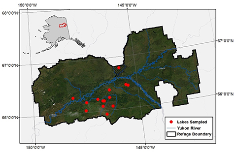
Figure 1. Map of the studied region. Lakes were sampled in the Alaskan Yukon Flats Basin (YFB) during winter, all but one lake is located within the boundary of the Yukon Flats National Wildlife Refuge. The inset map shows the state of Alaska with the sampled area outlined in red.
Download figure:
Standard image High-resolution imageA total of 13 lakes were sampled by float plane to measure under ice conditions in April 2017. Sampling reflects late winter conditions, since ice-cover typically initiates in October to November, and ice melt begins in May (late May, in 2017). Water temperature, pH, dissolved oxygen (DO) concentrations and fraction saturation were measured with a Yellow Springs Instruments EXO II probe. Sensors were calibrated before and after sampling and no drift in outputs were observed. Lake surface elevations were obtained from Google Earth. Lake depth values were taken from Bogard et al (2019), as the maximum depth at sampling sites. Water from pelagic regions of each lake was collected for laboratory analyses and was pumped across a filter on site (0.45 μm capsule filters, Geotech Environmental Equipment). Samples for analysis of deuterium and oxygen isotopic composition of water were stored in the dark in 20 ml plastic bottles, filled to capacity free of air. Samples for dissolved CO2 and CH4 stable isotopic composition were collected in 60 ml syringes using the headspace equilibration technique following standard methods (Striegl et al 2012). The partial pressures of CO2 and CH4 in the water were measured on site using a Los Gatos Research (LGR) Ultraportable Greenhouse Gas Analyzer. Gases were stripped from water by pumping water continuously through a closed showerhead system. Equilibrated gases were circulated into the LGR in a closed loop system following the general setup of (Webb et al 2016).
2.2. Laboratory analyses
Filtered water was analyzed for DOC following (Aiken 1992). Ultraviolet absorbance and SUVA254 were measured following (Weishaar et al 2003). Samples for the isotopic composition of water were analyzed at the U.S. Geological Survey Reston Stable Isotope Laboratory in Reston, VA, USA, using standard methods (Reéveész et al 2008). Isotopic composition of dissolved gases was analyzed at the University of Washington using a Picarro G2201-I Isotopic Analyzer. Triplicate samples were collected and are reported here as average values. Equilibrated gas samples were directly injected into the Analyzer using the small sample introduction module 2. In some cases, samples with extremely high gas concentrations were diluted with ultra-pure Nitrogen (N2) to reach target concentrations. After testing to confirm no effect on isotopic signatures, N2 was also added to some samples in cases where sample volumes were less than the required 17 ml of gas. Standards of CO2 (31.48‰) and CH4 (−38.3 ‰) were injected prior to sample processing. Standards were also injected at the end of some runs, confirming that instrument drift did not occur. A systematic offset in δ13C-CH4 was corrected using a two-point calibration curve (y = 0.9578x—0.1791; r2 = 1).
Stable isotopic composition of both O and C are reported in the text using delta notation, in equation (1):
where Rsample and Rstandard are ratios of heavy to light isotopes (18O:16O or 13C:12C) in samples (Rsample) and in standards (Rstandard) of Vienna standard mean ocean water or Vienna Pee Dee Belemnite.
2.3. Numerical and GIS analyses
To depict lake positions in the landscape, we developed a map of the YFB region using ArcGIS 10.4 (ESRI). All statistical analyses were performed using R version 3.3.3 1.1.463 (R Development Core Team 2017). To assess the relationships between gas content, isotopic composition, and environmental properties (including lake depth, elevation, and physico-chemical properties), we first tested for normality using the Shapiro Wilks test, and used Spearman correlation analyses to evaluate relationships for variables with non-normal distributions. The Pearson correlation test was used on log10-transformed data when comparing CO2 and CH4 concentrations, and on comparisons with normal data distributions. To explore which methanogenic pathway dominated in lakes, we used Keeling plot and Miller Tans plot approaches to evaluate the approximate isotopic composition of freshly produced CH4 prior to oxidation in the lakes under ice (Pataki et al 2003, Miller and Tans 2003, Zobitz et al 2006). The Keeling plot involves using isotopic values and CH4 concentrations to find an isotopic source signature via the y-intercept. With the Miller-Tans plotting approach, the slope of the regression model obtained by plotting the product of δ13C and the concentration of either gas provides the average isotopic signature of CH4. Regression relationships were calculated using a major axis regression approach with the 'lmodel2' package (Legendre 2013), because both x and y variables are subject to measurement error. Based on this regression approach, two distinct lake groups were identified using the Keeling and Miller-Tans plots, and the between-group differences in CH4 sources were summarized with box plots and compared statistically with student t-tests.
The Keeling plot method is typically used in simple systems with initial certain background δ13C-CH4 and a single source added over time, and therefore not entirely transferable to cross-system surveys with variable sources and sinks of CH4. As such, the Keeling plot was only used to visually assess isotopic patterns. The Miller-Tans approach is more robust in cross-system applications because the test accounts for inconsistencies in background constants, and incorporates uncertainties and errors in the collection and analysis process (Miller and Tans 2003). From this approach, we cautiously interpreted potential differences in slopes (i.e. source CH4 isotopic composition) among identified lake groupings. To ensure these applications were as accurate as possible, we restricted our explorations to periods of ice cover for two key reasons that simplify our interpretation of sources and sinks, and thereby make this approach more appropriate: First, during lake capping by ice, CH4 from individual loss pathways (diffusive, ebullitive) are trapped and homogenized in the water column (Elder et al 2019), enabling clear source identification. Second, sampling during ice cover eliminated the second potential removal pathway of CH4 (atmospheric loss), and thus we assume only microbial oxidation removed CH4 from lakes. This simplification of source and sink pathways helps to ensure our interpretation of isotopic composition was as accurate as possible. Still, we only qualitatively interpret these outcomes (i.e. using lake groupings).
3. Results and discussion
3.1. Extreme under ice variability of CO2 and CH4 content
Across our 13 sample lakes, partial pressures of CO2 and CH4 under ice were not normally distributed (figure 2, table 1), with CH4 having a more skewed distribution than CO2. CO2 content ranged from 454 to 19 000 μatm with a mean of 6673 μatm and a median of 5300 μatm, and CH4 content ranged from 1.60 to 29 000 μatm with a mean of 7040 μatm and a median of 1152 μatm. We observed a weak positive correlation between the log10 transformed CO2 and CH4 (figure 2; p= 0.18, r= 0.39). This relationship improved with the exclusion of an extreme outlier (Greenpepper Lake, Lake 6) (r= 0.72, p = 0.009). We present the data, however we suspect that this lake reflects a landscape position unique from others in this dataset, where it is perched within higher elevation conditions along the northern slopes of the White Mountain range. Furthermore, as outlined in Bogard et al (2019), this lake is shown to have the oldest mean DOC age (i.e. most depleted Δ14C signatures of DOC), and the most enriched values for the isotopes of water (table S1 (stacks.iop.org/ERL/15/105016/mmedia)), suggesting very little connection to the adjacent terrestrial and aquatic landscape.

Figure 2. Correlation between the partial pressures of CO2 and CH4 (n = 13). Note log10-scaled axes of plot. Outlier denoted by red star.
Download figure:
Standard image High-resolution imageTable 1. Key limnological and isotopic data associated with each lake (see table S1 for comprehensive dataset). Lakes are identified using unique numbers that are consistent throughout the paper. All abbreviations are defined in the text. All previously published datasets are openly available, as indicated in Bogard et al (2019). * denotes depths measured during previous open water sampling in spring.
| Lake I.D. | Surf. Elev. | Depth | DO | DO Sat. | pH | Chl a | pCO2 | pCH4 | δ13C-CO2 | δ13C-CH4 |
|---|---|---|---|---|---|---|---|---|---|---|
| m asl | m* | mg L−1 | % | μg L−1 | μatm | μatm | ‰ | ‰ | ||
| 1 | 134 | 12.8 | 5.93 | 40.8 | 7.77 | 8.92 | 3200 | 6.1 | −17.26 | −50.54 |
| 2 | 122 | 2 | 1.93 | 13.2 | 7.8 | 30.84 | 3460 | 20 700 | −13.68 | −58.09 |
| 3 | 120 | 2.2 | 0.9 | 6.3 | 7.47 | 12.95 | 5660 | 2700 | −19.52 | −69.85 |
| 4 | 136 | 5.6 | 3.09 | 22.3 | 7.5 | 10.78 | 5300 | 572 | −17.03 | −24.61 |
| 5 | 117 | 1.5 | 1.41 | 9.8 | 7.53 | 13.69 | 17 000 | 28 000 | −16.07 | −58.25 |
| 6 | 204 | 7 | 3.56 | 24.6 | 8.83 | 12.68 | 454 | 1324 | −15.31 | −29.62 |
| 7 | 226 | 6.5 | 9.05 | 62.7 | 8 | 3.74 | 2560 | 10.6 | −16.87 | −53.91 |
| 8 | 127 | 4.5 | 3.08 | 21.1 | 7.8 | 8.47 | 4100 | 3.7 | −16.23 | −50.2 |
| 9 | 102 | 1.8 | 1.09 | 7.6 | 7.98 | 51.74 | 7500 | 8150 | −20.41 | −71.87 |
| 10 | 146 | 1.5 | 1.44 | 9.9 | 6.83 | 11.86 | 19 000 | 29 000 | −10.18 | −58.09 |
| 11 | 303 | 4.6 | 9.56 | 66.3 | 7.26 | 9.03 | 3125 | 1.6 | −22.16 | −41.39 |
| 12 | 108 | 2 | 2.16 | 15.6 | 7.62 | 1.84 | 6000 | 36 | −18.29 | −19.59 |
| 13 | 126 | 3.7 | 1.25 | 8.7 | 7.16 | 5.53 | 9400 | 1152 | −23.02 | −33.85 |
Like many other studies in the northern circumpolar region, all lakes studied here were supersaturated in CO2 and CH4 (Elder et al 2018, Serikova et al 2019), but the range in under ice gas concentrations was among the most extreme in the literature. The pCO2 range across the lakes (454 to 19 000 μatm) spans beyond the range reported in a recent comprehensive survey of under ice pCO2 in Swedish lakes (median = 2961, 95% C.I. = 919 to 11 162 μatm (Denfeld et al 2016). Yet Striegl et al (2001) found that lakes in north-temperate U.S. had under ice pCO2 values reaching as low as 85 μatm, indicating that the low-end values observed in YFB lakes is not anomalous, and within the expected range of late winter CO2 content. All but one lake had CO2 concentrations exceeding CH4, which is a general trend in many northern lake regions and across distinct seasons (Anthony et al 2014, Rasilo et al 2015, Elder et al 2018, Denfeld et al 2018). The range in under ice pCH4 was also extreme, spanning 1.8 to 29 000 μatm. Very wide ranges in under ice CH4 content have been shown for other Alaskan lakes (Kling et al 1992, Sepulveda-Jauregui et al 2015, Elder et al 2018). Yet, CH4 content was heterogeneous (more so than for CO2) with only four lakes having concentrations >5000 μatm (figure 2). Heterogeneity of under-ice CH4 content is commonly observed, making it difficult to predict patterns and controls on winter CH4 accumulation (Denfeld et al 2018) as opposed to open water periods, where ice-free ebullition rates scale with incoming solar radiation (Wik et al 2014). Overall, despite the small regional area covered in our study, we still observed GHG gradients similar to those in more extensive geographic surveys in other regions (Townsend-Small et al 2017, 2018, Elder et al 2019). This heterogeneity, even within a localized survey of lakes, underscores the need to better define the mechanistic controls of GHG content in lakes in winter.
3.2. Environmental correlates of under ice CO2 and CH4 concentrations
Across an elevation range from 102 to 303 m asl, we observed a strong, non-linear relationship between GHG content and lake elevation. The highest concentrations of CO2 and (to a lesser extent) CH4 were found in lakes located below 150 m asl, situated closer to the Yukon River (figures 3(a) and (b); CO2: p = 0.03403, ρ = −0.6; CH4: p = 0.1516, ρ = −0.42). Only three lakes were located at elevations >150 m asl, though none of these sites had CO2 or CH4 content above ∼5000 μatm (figures 3(a) and (b)). In addition to elevation, we also examined hydrologic connectivity using δ18O-H2O as a proxy. Overall, many of the lakes exhibited enriched values of δ18O-H2O, from −18.67 to −10.36‰, indicating the dominance of evaporative processes in many lakes during ice free periods. Lakes with stronger connections to hydrologic networks (rivers, groundwater) are more depleted in δ18O-H2O with values corresponding to approximately −21‰ for river and groundwater and −27‰ for snow and permafrost (Anderson et al 2013, Halm and Griffith 2014). The enriched isotopic values observed here further indicate the lakes are weakly connected to hydrologic flows, we found no clear relationship between δ18O-H2O values and either pCO2 (p= 0.28, ρ= −0.32) or pCH4 (p= 0.64, ρ = 0.14).
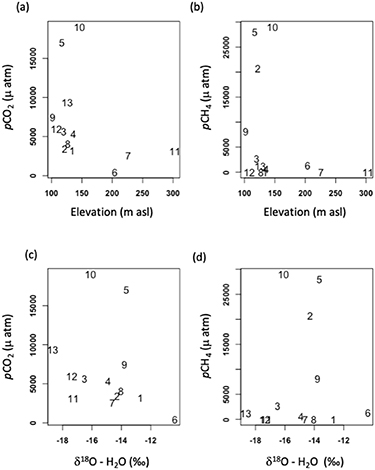
Figure 3. Relationship between the partial pressure of CO2 or CH4 and lake surface elevation (a, b) and hydrological connectivity (c, d). Lakes with stronger connections to hydrologic networks (rivers, groundwater) have more negative water isotopic values, while those with weaker hydrologic connections have greater water isotopic values.
Download figure:
Standard image High-resolution imageWe observed a wide range of relationships between under-ice gas content and the limnological properties of each study lake (figure 4). Maximum depth at the sampling site (Zmax) ranged from 0.9 to >12 m (figures 4(a) and (b)), and GHG content scaled inversely with depth (CO2: p = 0.0005, ρ = −0.83, CH4: p = 0.006, ρ= −0.72). Concentrations of CH4 were ∼ 5 orders of magnitude higher in lakes that were <2 m deep, while pCO2 among lakes scaled more linearly with depth. DO concentrations in the lakes ranged from near anoxia to near saturated (0.9 to 9.56 mg L−1; figures 4(c) and (d)). For both CO2 and CH4, concentrations were much greater at lower DO content (CO2: p = 0.003, ρ = −0.78, CH4: p = 0.009, ρ= −0.71). Yet this relationship was less linear for pCH4, which declined dramatically in environments with >2 mg L−1 DO. Consistent with an earlier survey of northern lakes (Kortelainen et al 2006), we found no relationship between organic matter and CO2 content. There was a wide, cross-lake DOC concentration range (14.6 to 181 mg L−1), and although no relationship to pCO2 was observed, lakes with the greatest DOC concentrations tended to have the highest pCH4 values (figures 4(e) and (f)); (CO2: p= 0.34, ρ= 0.29; CH4: p =.004, ρ= 0.75). Not only the quantity, but the composition of dissolved organic matter ranged widely among lakes, as indicated by SUVA254 values spanning from 0.99 to 4.00 (figures 4(g) and (h)), yet values were uncorrelated with CO2 or CH4 content (CO2: p= 0.29, r =0.31; CH4: p= 0.91, r =0.03). When compared to pH (not shown), pCH4 showed no relationship (p = 0.26), and the weak correlation with pCO2 (p = 0.02, r = −0.64) likely reflected the direct effect of elevated CO2 concentrations on pH. Although algal biomass as chl a pigment concentration does not capture total ecosystem productivity (i.e. macrophyte and benthic algal growth), it provides a general indication of the wide range in trophic status of our study lakes (figures 4(i) and (j)). While not correlated with lake pCO2, pCH4 tended to increase in more productive lakes with higher chl a concentration.

Figure 4. Pressures of CO2 (a, c, e, g, i) and CH4 (b, d, f, h, j) are compared to lake physico-chemical properties. See text for definitions and statistical relationships.
Download figure:
Standard image High-resolution imageOverall, lake surface elevation (dictating the general position in the surveyed landscape) and depth appear as important controls determining in which lakes elevated CO2 and CH4 content is observed. It is likely that these controls over-rode the influence of factors of secondary importance, since the three most shallow lakes (lakes 5, 10, and in some cases 2; Table S1) appeared as outliers with extremely high GHG concentrations in relationships between GHG content and other predictors (DOC, SUVA254, chl a concentration). This importance of landscape position in structuring GHG content has been demonstrated in global-scale analyses (Lapierre et al 2012) and makes sense at the regional scale in the YFB, first because lake depths typically become shallower moving from steeper, high elevation terrain, to flatter, low elevation terrain (Heathcote et al 2015), and second because shallow lakes tend to have greater content of CO2 and CH4 under ice (Ducharme-Riel et al 2015b, Denfeld et al 2016, 2018). The absence of a correlation between GHG content and water isotopic signatures reflects the fact that many lakes in the YFB region have weak hydrologic connectivity to riverine or groundwater flows, and receive comparatively little terrestrial C input (Johnston et al 2019). The weak or absent relationship between overall DOC aromaticity (as SUVA254) and CO2 and CH4 (respectively; figure 4) is in line with the independence of under-ice GHG content from external C loading in many of the lakes (Bogard et al 2019). While elevated lake GHG content was primarily observed at low elevations, CH4 content was additionally dependent on lake trophic status (chl a content), and DOC availability, which likely enhanced winter respiration and oxygen depletion (figures 4(d) and (j)). These secondary controls likely made under ice pCH4 content even more heterogeneous at low elevations than pCO2. Taken together, the variability in under ice GHG content appears to track general environmental characteristics (lake surface elevation and depth) and (for CH4) lake trophic status, which are predictable features that could be used in future studies (with more extensive lake sampling) to build broader regional models of under ice GHG content and spring emissions at ice-out, as has been done in better-studied boreal landscapes (Guo et al 2020).
3.3. Stable isotopic composition of CO2 and CH4
When compared to partial pressures, the δ13C values of each gas revealed distinct cross-lake patterns for both CO2 and CH4 (table 1, figures 5(a) and (b)). Values of δ13C-CO2 were more constrained, ranging from −10.13 to −23.02‰, and showing no relationship to gas concentration (figure 5(a); p= 0.86, ρ= −0.05). Conversely, values for CH4 ranged widely, from −19.59 to −71.87‰, and pCH4 was correlated non-linearly to isotopic composition (figure 5(b); p= 0.051, ρ= −.55), with isotopic values most enriched, and increasing sharply at concentrations below ∼2400 μatm. We found no correlation between the isotopic composition of CO2 and CH4 (figure 5(c); p = 0.67, ρ = −0.13).
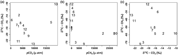
Figure 5. Stable isotopic composition of CO2 and CH4 compared with partial pressure of CO2 (a) and CH4 (b). Isotopic composition of each gas showed no clear relationship (c).
Download figure:
Standard image High-resolution image3.4. Exploring source CH4 composition across lakes
We used Keeling and Miller Tans plots (Keeling 1958, Miller and Tans 2003, Campeau et al 2017) to explore the potential source isotopic signature of fresh CH4 prior to microbial oxidation. CH4 is largely produced through two main pathways in freshwater ecosystems, where hydrogenotrophic methanogenesis generates CH4 with δ13C values from approximately −90‰ to −30‰, while the acetoclastic-derived source CH4 may range from −30‰ to −10‰ (Claus et al 2009). As detailed in the methods section, both plotting approaches use the concentration of methane and the δ13C-CH4 to predict the isotopic signature of source CH4. Using the Keeling approach (figure 6(a)), we plotted δ13C-CH4 values from each lake against the inverse of respective gas concentrations. Inverse values were log-transformed due to the extreme range and non-normal distribution of concentrations, therefore the intercept value of the regression model associated with the Keeling plot was not interpretable as the exact source value. Thus, we used this method in a more qualitative manner to compare lake categories. Major Axis (type-II) regression models applied in the Keeling plot showed two distinct groups of lakes (figure 6(a) group A: y = 16.48x-27.2, r2= 0.91, p = 0.0008; group B: y = 7.7x-63.5, r2= 0.96, p = 0.0006). Next, we used the Miller-Tans plotting approach to identify source isotopic signatures for CH4 in the two distinct lake groups identified with the Keeling plot. Here, the value of δ13C-CH4 was multiplied by the concentration of CH4, then compared to CH4 concentrations (figure 6(b)). Consistent with the Keeling plot groupings, lake distributions fell into two distinct groups (group A: y = −58.96x + 55.29, r2= 0.99, p <0.00001; group B: y = −71.8x + 2.2 29, r2= 0.99, p <0.00001).
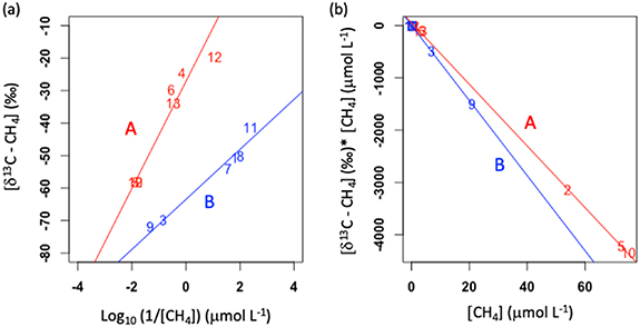
Figure 6. Qualitative assessment of source CH4 isotopic composition. (a) Keeling plot showing the relationship between δ13C-CH4 values and the log10 of the inverse of CH4 concentrations (1/[CH4]). We visually defined two distinct lake groupings (groups A and B). (b) A Miller-Tans plot with lake groupings A and B shown. In both panels, model 2 regression lines for groups A and B shown as red and blue, respectively, and statistics are reported in the text.
Download figure:
Standard image High-resolution imageThese two lake groupings in the Miller-Tans plots (figure 6(b)) indicate that lakes in the YFB appear to have a range of inputs from both acetoclastic and hydrogenotrophic pathways, with lakes in group B predominantly generating CH4 from the hydrogenotrophic pathway, and lakes in group A reflecting a mix of both CH4 source input pathways and increased relative importance of acetoclastic methanogenesis. This wide range in isotopic composition of δ13C-CH4 is consistent with other northern lake studies that showed a mix of pathways possibly supporting lake CH4 accumulation and processing via oxidation. In Eastern Canadian Arctic thermokarst lakes, hypolimnetic δ13C-CH4 signatures also ranged across lakes from −47.1 to −67.0 ‰, likely sourced from multiple pathways (Matveev et al 2018). In an unrelated study of Alaskan lakes, Elder et al (2018) used similar isotopic methods to show that under ice δ13C-CH4 ranged from −38.8‰ to −73.3‰. Acetoclastic methanogenesis uses acetate as a reactant to produce CH4 and CO2. Hydrogenotrophic methanogenesis produces CH4 through CO2 reduction. Therefore, differences in net CO2 production and consumption linked to methanogenesis in lakes of groups A and B could hypothetically alter the overall winter GHG budgets of the lake groups. Although there was no clear distinction in GHG content between the two groups of lakes with distinct isotopic signatures of fresh CH4 (i.e. signature prior to oxidation), generally the highest concentrations of CO2 and CH4 were found in those lakes that appear to produce CH4 primarily through the acetoclastic pathway, most notably in lakes 5 and 10 (figure 6(b)).
3.5. Methanogenic pathway dominance across environmental conditions
We categorized the lakes by their identified groups (A, B; figure 6), and explored whether lake and landscape features differed among groups. Lakes with isotopically depleted source CH4 dominated by hydrogenotrophic methanogenesis were found across the elevational gradient but on average, were located at higher elevation than lakes with enriched source CH4 (figure 7(a); t = −9.3, p < 0.0001). They were also often deeper (figure 7(c); t = 5.6, p < 0.0001), more oxygenated (figure 7(d); t = 6.1, p < 0.0001), had somewhat lower chl a concentrations (figure 7(g); t = 2.6, p = 0.02), and higher pH (figure 7(h); t = −31.5, p < 0.0001). While DOC concentrations were not different among groups (figure 7(e); t = −0.9, p = 0.39), and SUVA254 was uncorrelated to pCH4 across lakes (figure 4(h)), we found a significant difference in SUVA254 among the two lake groups. Group A lakes (isotopically enriched source CH4) had less aromatic organic matter, as inferred from somewhat lower SUVA254 values (figure 7(f); t = −3.7, p = 0.001). The differences among both groups in terms of hydrologic connectivity were statistically significant, but variable (figure 7(b); t = 25.9, p < 0.0001). Taken together, it appears that the dominance of individual methanogenic pathways may vary in a predictable way during winter months for lakes in the YFB region. These landscape patterns in CH4 isotopic composition (figure 7) generally makes sense, since hydrogenotrophic methanogens are often more O2-tolerant than obligate anaerobe acetoclastic methanogens (Oremland and Capone 1988, Zehnder 1988, Whiticar 1999), and declining pH can favor acetoclastic over hydrogenotrophic pathways (Conrad 2020). Differences in SUVA254 and chl a concentration also may reflect the fact that more productive environments rich in bio-labile organic matter can support higher relative rates of acetoclastic methanogenesis, while decomposition of complex aromatic materials favours hydrogenotrophic pathways (Conrad 2020).

Figure 7. Comparing lake properties among the two distinct lake groups of differing CH4 source dominance, identified using the Keeling and Miller-Tans Curve Approaches (figure 6). The lake groupings were used to explore differences in (a) surface elevation, (b) δ18O-H2O signature, (c) depth at the sampling site, (d) DO concentration, (e) DOC concentration, (f) SUVA254 value, (g) chl a concentration, and (h) pH. Both DO and DOC values were log10-transformed.
Download figure:
Standard image High-resolution image
3.6. Implications and summary
The winter ice-covered period represents an extended period of time for which we currently have a weak understanding of northern lake C biogeochemistry (Denfeld et al 2018). Here, we show that the patterns of winter under ice CO2 and CH4 content are heterogeneous across a suite of boreal lakes spanning a landscape gradient in interior Alaska, and that divergent stable isotopic signatures of CH4 indicate a potential contribution from different biogeochemical pathways. Therefore, these observations fill a critical gap in our understanding of C cycling in remote and understudied arid, flat, and circumpolar lake landscapes (Bogard et al 2019). The content of GHGs under ice in winter is extremely variable, with concentrations ranging from near- atmospheric equilibrium to extreme supersaturation. The degree of inter-lake variability in winter CO2 content shown for the YFB region is consistent with observations from other boreal and temperate lakes (Ducharme-Riel et al 2015a). This variability may lead to a wide range in importance (in an annual context) of early-spring emissions pulse at ice out, from one lake to the next, though such an exercise is beyond the scope of this research. While this variability complicates our ability to predict region-wide emissions pulses at ice out, the observed correlations between lake properties (Zmix, DO, DOC, SUVA), and catchment properties (elevation, δ18O-H2O) suggests there is potential for future studies to empirically model lake CO2 emissions at ice-out in the YFB or similar landscapes. We also found a comparably wide range in CH4 concentrations in YFB lakes. Here, the much weaker relationship between CH4 and lake or catchment properties suggests that the construction of comparable models to predict the CH4 pulse at ice out will be more difficult for the YFB region (but see Guo et al 2020). More detailed sampling is likely needed to constrain these relationships. The fact that under ice CO2 and CH4 content was positively correlated in most lakes, and gas content was highest at lowest elevation in the region, provides a first step to constraining the potential locations for emissions hotspots during spring thaw. Overall, because of the limitations on sampling in the winter in these remote regions (mostly due to lack of access), our results add critical data to fill a major gap in our understanding of winter limnology and C biogeochemistry.
To date, few studies have employed stable isotopic surveys of lake GHGs that build up under ice, especially for CH4 (Townsend-Small et al 2017, 2018, Elder et al 2019). Here we demonstrate that even within a small geographic region, the importance of individual biochemical pathways supporting winter CH4 content and emissions at ice-out can vary greatly from one lake to the next. Such differences in methanogenic pathway dominance may have consequences for the overall radiative effect of lake emissions, because acetoclastic and hydrogenotrophic methanogenesis pathways respectively consume and produce CO2. While our survey provides a first-order exploration of potential differences in the relative importance of these pathways, more detailed isotopic and microbial studies are needed to constrain the overall contributions from these distinct pathways, relative to oxidation of CH4. Furthermore, the extreme range in isotopic signatures of CH4 under ice, even in the limited geographic region surveyed here, indicate that it will be exceedingly difficult to distinguish lake emissions from other sources (terrestrial, riverine) at spring thaw using airborne technologies and top-down isotopic surveys.
There remains much to be learned regarding the patterns and controls of under ice GHG accumulation in boreal and arctic lakes. More research must be done to formally construct accurate C budgets (Denfeld et al 2018), and to better define the mechanisms regulating net GHG accumulation. Here, our study was designed to target the latter issue. Our isotopic evaluation of CH4 composition, and our correlations between under ice GHG content and environmental variables both fill an important research gap related to winter C cycling in lakes from this understudied arid, low-relief region that is representative of up to a quarter of northern high-latitude lake landscapes worldwide.
Acknowledgments
This project was supported by funding provided to DEB from the University of Washington and the U.S. Geological Survey and National Aeronautics and Space Agency (NASA-ABoVE Project 14-TE14-0012), to RGS from the U.S. Geological Survey Climate and Land Use Change and Water Mission Areas, and to MJB from the Canada Research Chairs program and the University of Lethbridge. The authors thank Fenix Garcia Tigreros Kodovska and four anonymous reviewers for their comments that improved earlier versions of this manuscript.
Data availability statement
All data that support the findings of this study are included within the article (and any supplementary information files). All previously published data used here are openly available from the original publications.