

Abstract
We present a gridded inventory of Mexico's anthropogenic methane emissions for 2015 with 0.1° × 0.1° resolution (≈10 × 10 km2) and detailed sectoral breakdown. The inventory is constructed by spatially allocating national emission estimates from the National Inventory of Greenhouse Gases and Compounds constructed by the Instituto Nacional de Ecología y Cambio Climático (INECC). We provide additional breakdown for oil/gas emissions. Spatial allocation is done using an ensemble of national datasets for methane-emitting activities resolving individual municipalities and point sources. We find that emissions are highest in central Mexico and along the east coast, with substantial spatial overlap between major emission sectors (livestock, fugitive emissions from fuels, solid waste, and wastewater). Offshore oil/gas activities, primarily oil production, account for 51% of national oil/gas emissions. We identify 16 hotspots on the 0.1° × 0.1° grid with individual emissions higher than 20 Gg a−1 (2.3 tons h−1) including large landfills, offshore oil production, coal mines in northern Mexico, a gas processing complex, and a cattle processing facility. We find large differences between our inventory and previous gridded emission inventories for Mexico, in particular EDGAR v5, reflecting our use of more detailed geospatial databases. Although uncertainties in methane emissions remain large, the spatially explicit emissions presented here can provide the basis for inversions of atmospheric methane observations to guide improvements in the national inventory. Gridded inventory files are openly available at (https://doi.org/10.7910/DVN/5FUTWM).
Export citation and abstract BibTeX RIS

Original content from this work may be used under the terms of the Creative Commons Attribution 4.0 license. Any further distribution of this work must maintain attribution to the author(s) and the title of the work, journal citation and DOI.
1. Introduction
Methane emissions originate from a range of anthropogenic sectors [1]. Reducing these emissions is important for achieving climate goals because methane is a major greenhouse gas [2–6]. Under the Paris Agreement, each country must outline its emissions reduction strategies for greenhouse gases in Nationally Determined Contributions (NDCs) or Intended Nationally Determined Contributions (INDCs). Methane mitigation measures for the fossil fuel and waste sectors have been incorporated into many NDCs and INDCs because they can be achieved at low economic cost using currently available technologies [4, 6–8].
Mexico accounts for about 2% of global anthropogenic methane emissions [9], and its INDC has committed to a 22% reduction in greenhouse gas emissions by 2030 relative to a business-as-usual (BAU) projected growth with a baseline of 2013 emissions [10]. Under this INDC, Mexico plans to reduce oil/gas methane leakage emissions by 25%, and to recover the methane emitted from solid waste landfills and wastewater treatment plants [11]. Mexico also joined Canada and the US in the North American Climate, Clean Energy, and Environment Partnership in 2016 which includes commitments to reduce oil/gas methane emissions by 40%–45% by 2025 relative to 2012 levels, and to implement national reduction strategies for other methane sources [12]. Mexican federal regulations to curb methane emissions from the oil/gas sector were published in 2018 [13] and have now transitioned to the implementation and compliance phase which has created a need for accurate tracking of emissions.
Mexico's anthropogenic methane emissions are estimated by the Instituto Nacional de Ecología y Cambio Climático (INECC) and the Secretaría de Medio Ambiente y Recursos Naturales (SEMARNAT) as part of the National Inventory of Greenhouse Gases and Compounds [14] which we will refer to hereafter as the national inventory. The most recent version of the national inventory (extending to 2015) forms a part of Mexico's Sixth National Communication [15] reported to the United Nations Framework Convention on Climate Change (UNFCCC) and used to track progress toward INDC goals. Most of Mexico's emissions are estimated using the default Tier 1 methods from the Intergovernmental Panel on Climate Change (IPCC) with generic emission factors [16], introducing a large degree of uncertainty for some sectors. For example, Mexico's methane emissions from oil and gas have 56% and 40% uncertainty, respectively, according to the national inventory [14].
Observations of atmospheric methane can provide independent information to test and improve emission inventories through inverse analyses [17–19], but they require prior estimates of the spatial distribution of emissions in order to interpret the observed gradients of atmospheric concentrations [18]. EDGAR has been the go-to choice for these prior estimates because it is the only comprehensive global inventory with fine spatial (0.1° × 0.1°) information [20], but evaluation for the US shows that it has large errors [21, 22]. National inventories reported to the UNFCCC often use country specific emission factors and industry reported activity data, but they are generally missing the necessary spatial information as is the case for Mexico. Previous studies have produced spatially explicit (gridded) versions of national inventories for Australia [23], Switzerland [24], the United States [21], the United Kingdom [25], and for fuel exploitation globally [26]. A major advantage in using the national inventories as prior estimates in inversions of atmospheric data is that discrepancies identified by the inversions are directly relevant to improving the inventories and therefore inform climate policy.
Here we create a spatially explicit version of Mexico's national inventory at 0.1° × 0.1° resolution (≈10 × 10 km2) including detailed breakdown by source sectors (see the data availability section). Our prime motivation is to provide a prior estimate for inversions of atmospheric observations that may guide improvements in the national inventory and better inform INDC targets. We identify specific hotspots to serve as targets for atmospheric observations. The spatial allocation of emissions presented here can also serve policy analysis and assessments at the national, state, and municipal levels.
2. Methods
2.1. National inventory for Mexico
Table 1 gives the anthropogenic methane emissions from Mexico's national inventory for 2015 as reported to the UNFCCC [14]. Here and elsewhere, we refer to sectors as the primary entries in table 1 (e.g. Fuel combustion activities) and subsectors as the secondary entries (e.g. Road transportation). Figure 1 displays the relative contributions of major sectors and subsectors. Total national emission is 5.1 Tg a−1 with dominant sectoral contributions from livestock (47%), fugitive emissions from fuels (20%), solid waste management and disposal (15%), and wastewater treatment and discharge (14%).

Figure 1. Relative contributions of individual sectors (inner ring) and subsectors (outer ring) to Mexico's anthropogenic methane emissions in 2015 as estimated in the national inventory [14]. Absolute contributions are in table 1.
Download figure:
Standard image High-resolution imageTable 1. Anthropogenic methane emissions from Mexico in 2015
| Sector/subsector | Emission Gg a−1 | Uncertainty
% | Category code |
|---|---|---|---|
| Fuel combustion activities | 99.9 | — | 1A |
| Road transportation | 11.3 | 81.4 | 1A3b |
| Residential | 77.3 | 4.9 | 1A4b |
| Other combustion |
11.3 | — | — |
| Fugitive emissions from fuels | 1032.7 | — | 1B |
| Underground coal mining | 275.6 | 37.6 | 1B1ai |
| Surface coal mining | 2.5 | 66.0 | 1B1aii |
| Oil—leakage, venting |
185.1 | 56.5 | 1B2ai,1B2aiii |
| Gas—leakage, venting |
317.6 | 39.7 | 1B2bi,1B2biii |
| Oil and gas—flaring |
251.9 | — | 1B2aii,1B2bii |
| Chemical industry | 6.5 | — | 2B |
| Petrochemical and carbon black production | 6.5 | 36.9 | 2B8 |
| Livestock | 2361.8 | — | 3A |
| Enteric fermentation—cattle | 1790.0 | 6.5 | 3A1a |
| Enteric fermentation—sheep | 43.6 | 9.7 | 3A1c |
| Enteric fermentation—goats | 43.5 | 10.1 | 3A1d |
| Enteric fermentation—other animals |
31.4 | — | - |
| Manure management—cattle | 284.6 | 6.4 | 3A2a |
| Manure management—pigs | 158.3 | 7.3 | 3A2h |
| Manure management—other animals |
10.4 | — | — |
| Aggregate sources | 36.6 | — | 3C |
| Biomass burning—forests | 5.8 | — | 3C1a |
| Biomass burning—croplands | 24.0 | 241.1 | 3C1b |
| Biomass burning—grasslands | 0.9 | — | 3C1c |
| Rice cultivation | 5.9 | 55.8 | 3C7 |
| Solid waste disposal | 782.9 | — | 4A |
| Managed waste disposal sites | 607.4 | 3.5 | 4A1 |
| Unmanaged waste disposal sites | 87.7 | 2.4 | 4A2 |
| Open dumpsites for waste disposal | 87.7 | 0.8 | 4A3 |
| Biological treatment of solid waste | 4.2 | 104.4 | 4B |
| Incineration/open burning of waste | 22.1 | — | 4C |
| Waste incineration | <0.1 | 6.5 | 4C1 |
| Open burning of waste | 22.1 | 97.6 | 4C2 |
| Wastewater treatment and discharge | 729.8 | — | 4D |
| Domestic wastewater | 133.1 | 7.6 | 4D1 |
| Industrial wastewater | 596.7 | 5.2 | 4D2 |
| Total | 5076.5 | 4.9 | — |
aEmissions are from Mexico's National Inventory of Greenhouse Gases and Compounds [14] as reported to the UNFCCC. bSector names, subsector names, and category codes match those in IPCC guidelines [16], and subsector breakdown matches the national inventory except for the aggregation of subsectors with very low emissions. cUncertainties are from Mexico's national inventory and reported as ±2σ relative error standard deviations. Dashes indicate sectors/subsectors for which uncertainty data are not available. dIncluding sources from the energy industry (1A1), manufacturing and construction (1A2), transport (1A3 not including 1A3b), commercial/institutional (1A4a), and agriculture/forestry/fishing (1A4c) subsectors. eFurther disaggregated in table 2. fHorses, mules and asses, and pigs. gSheep, goats, horses, mules and asses, and poultry.
Table 2 provides additional breakdown for oil/gas emissions by source type based on information embedded in the national inventory [14]. This additional breakdown is necessary for the implementation of mitigation measures and to track the effectiveness of existing oil/gas regulations in Mexico.
Table 2. Disaggregation of oil/gas methane emissions by source type
| Source type | Leakage Gg a−1 | Uncertainty
% | Venting Gg a−1 | Uncertainty
% | Flaring Gg a−1 | Uncertainty
% |
|---|---|---|---|---|---|---|
| Oil | 4.6 | — | 180.5 | — | 250.1 | — |
| Exploration | 0 | — | <0.1 | −90, +100 | <0.1 | −90, +100 |
| Production | 0.1 | −96, +96 | 178.4 | −66, +66 | 240.1 | −12, +12 |
| Transport | 0.5 | −90, +100 | 1.8 | −90, +100 | <0.1 | −88, +123 |
| LNG terminals | 3.1 | −90, +100 | 0.2 | −90, +100 | — | — |
| Refining | 0.9 | −90, +200 | <0.1 | −54, +111 | 10.0 | −70, +70 |
| Distribution | 0 | — | — | — | — | — |
| Gas | 203.5 | — | 114.3 | — | 1.8 | — |
| Exploration | 0 | — | 0.1 | −90, +100 | <0.1 | −90, +100 |
| Production | 37.5 | −53, +53 | 83.9 | −90, +100 | - | — |
| Processing | 71.2 | −90, +100 | <0.1 | −66, +66 | 1.8 | −76, +137 |
| Transmission |
45.4 | −90, +100 | 30.2 | −75, +75 | — | — |
| Distribution | 49.4 | −90, +100 | — | — | — | — |
aSource type emissions are estimated by taking the oil/gas subsector totals in table 1 and further disaggregating them using information embedded in Mexico's national inventory [14]. bUncertainties are from the national inventory and reported as (−2σ, +2σ) relative error standard deviations. cIncludes storage emissions but they are estimated to be negligible.
The national inventory has no intra-annual variability and we do not introduce any in our gridded inventory. Seasonal variability is expected to be small except for manure emissions, which can be distributed over the year on the basis of local temperature [21]. Emissions from rice cultivation are seasonal [27] but are very small in Mexico.
2.2. Spatial allocation of national inventory
We spatially allocate the national inventory emissions to a 0.1° × 0.1° grid using a number of datasets with national coverage, most of which can be accessed via the federal government's online data portal (https://datos.gob.mx, last access: January 2020). We rely heavily on Mexico's Directorio Estadístico Nacional de Unidades Económicas (DENUE) which includes the point locations of major industrial and commercial facilities [28], and for oil and gas we primarily use the Sistema de Información de Hidrocarburos (SIH) which includes geospatial information for a majority of Mexico's oil and gas infrastructure [29]. Additional details on the spatial datasets used are included in the relevant sections below.
For methane point sources we distribute emissions using either the number or the activity of individual facilities. For non-point sources we distribute emissions using the count of sources per grid cell (e.g. number of cows) or categorical information (e.g. source present or not in the grid cell). For some subsectors we first estimate state or municipal emissions and then allocate to finer scale if possible. Mexico has 32 states subdivided into 2465 municipalities.
2.2.1. Fuel combustion activities and chemical industry.
Road transportation emissions are allocated to road networks according to road length [30]. Residential and commercial emissions are allocated by urban population [31]. Combustion emissions associated with all other activities, including electricity generation, are allocated uniformly to facilities that associate with the relevant economic activity in the DENUE dataset. Petrochemical and carbon black production emissions are allocated uniformly to petrochemical facilities in DENUE.
2.2.2. Fugitive emissions from fuels.
Emissions from underground and surface coal mining are allocated to coal mining facilities in DENUE and weighted by coal production per municipality [32].
We first separate well and non-well emissions so we can allocate well emissions by oil or gas production per well. We estimate that 89% of oil production emissions occur at wells and 11% occur at non-well production facilities (e.g. oil batteries) based on the number of each type of facility in the SIH database [29]. For gas production emission we estimate that 57% occur at wells, 39% at non-well facilities, and 4% along gathering pipelines based on the partitioning of natural gas system emissions in Annex 3.6 (table 3.6–1) of the U.S. EPA Inventory of Greenhouse Gas Emissions and Sinks (GHGI) [33]. Oil/gas production emissions from wells and exploration emissions (well drilling and completion) are allocated to well locations in the SIH database weighted by oil or gas production per well for 2015 [34]. Non-well oil/gas production emissions are allocated to non-well facilities and gathering pipelines in the SIH database using facility count and pipeline length, respectively.
Oil transport emissions related to pipelines (including liquified petroleum gas) are allocated to SIH oil pipelines by pipeline length, and oil transport emissions related to oil cargo loading are allocated to the locations of ports [28]. Oil refining emissions are allocated to refineries according to refinery production capacity in the SIH database. Emissions from liquified natural gas (LNG) are allocated to the locations of LNG terminals [35]. Gas processing emissions are allocated uniformly to SIH processing facilities. We assume based on the GHGI (again, Annex 3.6) that 86% of gas transmission emissions occur at compressor stations and allocate these emissions uniformly to SIH compressor stations. The remaining 14% of gas transmission emissions are allocated to SIH gas pipelines by pipeline length. Emissions from gas distribution to end users are allocated to states using the volume of gas consumed by residential and commercial users [36], and state emissions are then allocated by urban population density [31].
2.2.3. Livestock and aggregate sources.
Manure management and enteric fermentation emissions are allocated to municipalities based on animal counts [37] and restricted to pastureland, agricultural land, and scrubland [38] with the exception that we do not have municipal data for horses, mules, and asses (<1% of livestock emissions) so we uniformly allocate these emissions to the appropriate land types. Forest and grassland biomass burning emissions are allocated to municipalities using burned area [39] and restricted to forests, pastureland, and scrubland [38], while for croplands we use the harvested weight per municipality of the major residue burning crops [40] (wheat, sorghum, alfalfa, corn, barley, grain, rice, cotton, and sugar cane [41, 42]) and restrict emissions to agricultural land. For rice cultivation we use the harvested weight of rice per municipality [40] and restrict emissions to agricultural land.
2.2.4. Solid waste disposal.
Managed waste disposal (landfill) emissions are allocated to managed solid waste disposal sites provided by INECC using the weight of waste in place at each site. For the sites with known point locations we restrict site emissions to the grid cell containing the site (84% of emissions), and for the sites without known locations (16% of emissions) we allocate site emissions uniformly to the municipality containing the site. The same approach is taken for unmanaged disposal sites (71% of emissions to sites with known point locations) and open dumpsites (80% of emissions to sites with known point locations).
2.2.5. Biological treatment of solid waste and incineration/open burning of waste.
Emissions from biological treatment of solid waste are allocated to municipalities using the weight of solid waste treated per municipality [43]. Waste incineration emissions are allocated to the locations of permitted facilities [44], and emissions from open burning of waste are allocated by population [31].
2.2.6. Wastewater treatment and discharge.
Treatment of domestic wastewater accounts for 55% of domestic wastewater emissions [14]. These emissions are distributed to wastewater treatment plants according to data from the Comisión Nacional del Agua (CONAGUA) [45] on the average daily flow at each plant and the method of wastewater treatment which affects the magnitude of emissions. The remaining 45% of domestic wastewater emissions are from discharges of untreated wastewater and are allocated by population density [31] weighted by the number of untreated wastewater discharge sites per municipality [43].
Treatment of industrial wastewater accounts for 13% of industrial wastewater emissions [14]. INECC provided a breakdown of these emissions by industry, and we allocate these emissions to municipalities using the average daily wastewater flow at industry-specific wastewater treatment plants per municipality provided by INECC (the data were provided to INECC by CONAGUA through an official request). We do not have wastewater treatment plant data for some industries so we allocate these emissions uniformly to the appropriate industrial facilities in DENUE [28]. The remaining 87% of industrial wastewater emissions are from discharge of untreated wastewater. We allocate these emissions to states using the volume of untreated wastewater generated annually per state. We estimate this volume by finding the difference between the total water volume supplied to industry as indicated by water usage permits in the Registro Público de Derechos de Agua (REPDA) [46] and the total volume of industrial wastewater treated in wastewater treatment plants [47]. We then allocate state emissions to municipalities using the volume of water used by industry per municipality as indicated by REPDA permits in 2015 [48].
3. Results
3.1. Spatial distribution of emissions
Figure 2 shows the spatially allocated total emissions from Mexico's national inventory for 2015, and the sectoral contributions from livestock, fuels, solid waste disposal, and wastewater, accounting for over 97% of total emissions. Total emissions are highest in central Mexico and along the east coast, reflecting contributions from all four sectors.
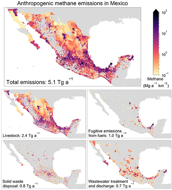
Figure 2. Total and sectoral anthropogenic methane emissions from Mexico in 2015. The emissions are from Mexico's national inventory [14] and spatially allocated to a 0.1° × 0.1° grid. Emissions below 0.1 Mg km−2 a−1 are not shown. The four sectors shown here account for 4.9 Tg a−1 of Mexico's total anthropogenic methane emissions.
Download figure:
Standard image High-resolution imageLivestock emissions total 2.4 Tg a−1 with cattle enteric fermentation and manure management contributing 88% and pig manure management contributing 7%. Emissions are highest in central Mexico and along the east coast, reflecting dense livestock populations which we capture by restricting municipal livestock populations to the pasture and agricultural lands in these regions. Emissions are especially concentrated in the states of Jalisco, Durango, and Veracruz due to their large cattle populations with Jalisco and Veracruz having the greatest number of milk and beef cows in 2015, respectively.
Oil/gas emissions total 0.7 Tg a−1 with flaring and venting during oil production as the two largest sources accounting for 32% and 24% of oil/gas emissions, respectively. Emissions are concentrated along the east coast, and offshore activities account for 51% of oil/gas emissions. Emissions are highest in regions of intense oil production, reflecting our use of oil and gas production per well to allocate emissions. Coal emissions total 0.3 Tg a−1 and are concentrated in the state of Coahuila in northern Mexico.
Solid waste emissions total 0.8 Tg a−1. Managed waste disposal sites (landfills) contribute 78% while unmanaged sites and open dumpsites each contribute 11%. The spatial distribution of solid waste emissions reflects the facility locations we use to map emissions. These largely follow population density although landfill sites tend to be located on the peripheral of cities rather than in city centers. Emissions are highest in central Mexico where there are a number of large facilities. Hotspot facilities are discussed in section 3.2.
Wastewater treatment and discharge emissions total 0.7 Tg a−1 of which 28% are domestic and 76% are industrial. The spatial distribution of domestic wastewater emissions follows population density, reflecting both the locations of treatment plants and the discharge of untreated wastewater. Industrial wastewater emissions are spread out spatially based on the locations of industries associated with significant water usage and organic waste generation, in particular the food and beverage industries. Regions of high emissions include central Mexico, the Yucatán Peninsula, and the Baja California Peninsula. Emissions from domestic and industrial wastewater treatment plants are more concentrated than untreated wastewater discharges because we allocate emissions to specific facilities.
3.2. Emission hotspots
Figure 3 shows the hotspots in our inventory exceeding 20 Gg a−1 (2.3 tons h−1) per 0.1° × 0.1° grid cell. Table 3 gives the locations and magnitudes of these hotspots. There are 16 such hotspots, accounting together for 13% of national emissions. The largest hotspot is the Mina VII coal mine (1; 119 Gg a−1) of the MICARE Unit in Nava, Coahuila. Coal production in Nava accounts for 42% of Mexico's coal production, while the nearby municipality of Múzquiz (including hotspots 4, 8) accounts for 39% [32]. The second largest hotspot is the Neza III landfill just outside of Mexico City (2; 116 Gg a−1) which is surrounded by four additional landfill hotspots (11, 12, 14, 15). The third largest hotspot is from offshore oil/gas production in the Ku/Maloob/Zaap oil field (3; 81 Gg a−1) and is part of four clustered offshore emission hotspots (3, 6, 9, 10) that together account for 37% of national oil production and 29% of associated gas production in 2015 [34]. We also find large emissions from the nearby onshore Cactus gas processing complex (7; 28 Gg a−1). Other emission hotspots include landfills in Monterrey, Nuevo León (5; 34 Gg a−1) and Tijuana, Baja California (16; 20 Gg a−1), and the SuKarne cattle processing facility in Vista Hermosa, Michoacán (13; 21 Gg a−1).

Figure 3. Emission hotspots in our inventory, defined as 0.1º × 0.1º grid cells emitting over 20 Gg a−1 (2.3 tons h−1). Table 3 gives detailed information for each hotspot.
Download figure:
Standard image High-resolution imageTable 3. Emission hotspots in Mexico
| Rank | Facility(ies) | Location | Emission
(Gg a−1) |
|---|---|---|---|
| 1 | Mina VII coal mine | 28.37 N, 100.59 W | 119 |
| 2 | Neva III landfill | 19.42 N, 99.00 W | 116 |
| 3 | Ku/Maloob/Zaap offshore oil field (multiple) | 19.55 N, 92.5 W | 81 |
| 4 | Múzquiz coal mines (multiple) | 19.65 N, 101.35 W | 48 |
| 5 | SIMEPRODE landfill | 25.85 N, 100.30 W | 34 |
| 6 | Akal/Sihil offshore oil fields (multiple) | 19.45 N, 92.05 W | 30 |
| 7 | Cactus gas processing complex | 17.90 N, 93.19 W | 28 |
| 8 | Múzquiz coal mines (multiple) | 19.75 N, 101.35 W | 28 |
| 9 | Akal/Ixtoc/Kambesah/Ku/Kutz offshore oil fields (multiple) | 19.45 N, 92.15 W | 27 |
| 10 | Ku/Maloob/Zaap offshore oil field (multiple) | 19.55 N, 92.15 W | 27 |
| 11 | Tlalnepantla de Baz landfill |
19.58 N, 99.21 W | 23 |
| 12 | Tepatlaxco landfill | 19.49 N, 99.30 W | 23 |
| 13 | SuKarne cattle facility | 20.26 N, 102.44 W | 21 |
| 14–15 | Milagro/Cañada landfills (multiple) |
19.35 N, 98.85 W | 21 |
| 19.35 N, 98.75 W | 21 | ||
| 16 | Valle de las Palmas landfill |
32.41 N, 116.74 W | 20 |
aHotspots are defined as any 0.1° × 0.1° grid cell with emissions greater than 20 Gg a−1 in our inventory. The emissions may be dominated by a single facility, in which case the facility location is given; or by multiple facilities, in which case the location is the center of the grid cell. See figure 3 for a map of the hotspots labeled by rank. bTotal emission in the 0.1° × 0.1° grid cell. cAccounts for 75% of grid cell emission; additional smaller waste disposal sites account for the remaining 25%. dThe municipality for these two landfills is known (Ixtapaluca in the State of Mexico) but not the exact locations. The municipality encompasses two grid cells so we give the center of both grid cells. The two landfills combined emit an estimated 40 Gg a−1 which is uniformly distributed in the two municipal grid cells (the remaining 2 Gg a−1 of emissions are contributed by other sources in the grid cells).
3.3. Uncertainty estimates
Uncertainty estimates for national emissions by subsector are reported by INECC as ±2σ relative error standard deviations (table 1) [14]. For the oil/gas subsectors some uncertainty estimates are asymmetrical so they are reported as (−2σ, +2σ) relative error standard deviations (table 2). Uncertainties are relatively large (38%–66%) for the fuel subsectors but very small (<10%) for the other major emission subsectors including cattle enteric fermentation, cattle/pig manure management, managed solid waste disposal (landfills), and industrial wastewater, resulting in a very low uncertainty of 4.9% on the total national emission. The latter uncertainty is likely too low given that other North American countries estimate much higher subsector uncertainties. For example, the average uncertainty estimate (±2σ relative error standard deviations) for cattle enteric fermentation is 15%–20% for the US and Canada, while the manure management uncertainty estimate range is 19%–50% [33, 49]. Hristov et al [50] independently estimated an average uncertainty of 16% for US enteric fermentation emissions and 64% for manure management. The landfill and industrial wastewater uncertainties are also much higher for Canada and the US (∼40%–50%).
Our gridded inventory has additional uncertainty related to the spatial allocation of emissions. Maasakkers et al [21] evaluated their 0.1° × 0.1° gridded national inventory for the US with a more detailed 4 × 4 km2 inventory constructed by Lyon et al [22] for northeastern Texas including local information on sources and direct methane emission measurements. They found uncertainties (±1σ) of 50%–100% for all subsectors on the 0.1° × 0.1° grid. Uncertainties on some sources decreased with spatial averaging, in particular for livestock, but remained above 30% for all subsectors even at 0.5° × 0.5° spatial resolution. In absence of empirical estimates in Mexico similar to those of Lyon et al for evaluation of our inventory's spatial uncertainty we recommend using the Maasakkers et al relative uncertainty estimates for our gridded inventory.
The locations of our hotspots are well established, but there is uncertainty in the allocation of emissions between large facilities, especially when sources have skewed emissions distributions [51]. We are not able to capture hotspot emissions from conditions that may be related to abnormal operating conditions or anomalous activity [51, 52].
3.4. Comparison to previous emission inventories
Figure 4 compares Mexico's national inventory of anthropogenic methane emissions to EDGAR v5 [20] for 2015. EDGAR estimates a total emission of 6.7 Tg a−1, which is 25% higher than the national inventory. Livestock (2.8 Tg a−1) and wastewater (0.7 Tg a−1) emissions in EDGAR are similar to the national inventory. Solid waste disposal emissions (1.6 Tg a−1) are a factor of two greater, coal emissions (0.05 Tg a−1) are 81% lower, and oil/gas emissions (1.3 Tg a−1) are 78% higher. EDGAR uses global datasets of country activity data (e.g. the number of cattle) to calculate emissions, so these differences in sector emissions reflect the use of country-specific activity data and emission factors in Mexico's national inventory.
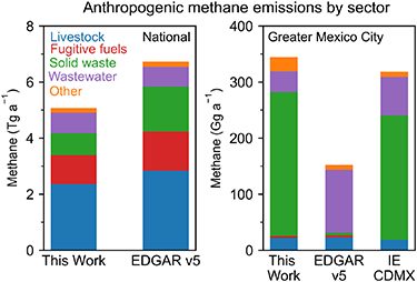
Figure 4. Anthropogenic methane emissions in Mexico (left) and Greater Mexico City (right). Results from this work are compared to EDGAR v5 [20] and to IE CDMX [53]. The Greater Mexico City domain is defined by IE CDMX and extends over (18.9 N—20.1 N latitude, 98.5 W—99.7 W longitude).
Download figure:
Standard image High-resolution imageAlso shown in figure 4 is a comparison to a 2016 emission inventory for the Metropolitan Area of the Valley Mexico, Inventario de Emisiones de la Ciudad de México (IE CDMX) [53]. This includes both Mexico City proper and surrounding municipalities. Total anthropogenic emission in that inventory is 319 Gg a−1, close to our inventory (344 Gg a−1) and much higher than EDGAR (152 Gg a−1). The IE CDMX inventory has 70% of its emission from solid waste, consistent with our inventory (74%), while EDGAR has 74% of its emission from wastewater.
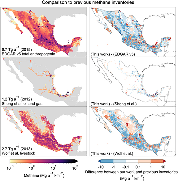
Figure 5 compares the spatial distribution of emissions in our work and EDGAR. Figure S1 (available online at stacks.iop.org/ERL/15/105015/mmedia) shows the comparison by sector. EDGAR livestock emissions are more diffuse which is likely due to our use of municipal livestock statistics. EDGAR wastewater emissions follow population whereas many of our high emission regions do not follow population because they are associated with industrial wastewater. The discharge of industrial wastewater to water bodies has been recognized as both a climate and water pollution concern in Mexico [54]. EDGAR's solid waste emissions are concentrated in fewer grid cells than our inventory likely because we include unmanaged sites and dumpsites. Offshore production accounts for only 16% of total oil/gas emissions in EDGAR but 51% in our inventory. Gas transmission emissions are concentrated at compressor stations in our work but are uniform along pipelines in EDGAR.
Figure 5. Emissions estimates for Mexico from previous gridded emission inventories. The left panels show total anthropogenic emissions in 2015 from EDGAR v5 [20], oil and gas emissions in 2012 from Sheng et al [55], and livestock emissions in 2013 from Wolf et al [56]. The right panels show the differences between our work and these previous inventories. All inventories are presented here at 0.1° × 0.1° resolution.
Download figure:
Standard image High-resolution image
EDGAR is also very different in the distribution and magnitude of emission hotspots. The two largest hotspots in EDGAR are landfills with grid cell emissions of 840 Gg a−1 and 420 Gg a−1, higher than any of our hotspots and not coincident spatially. The oil/gas hotspots in EDGAR have higher emissions (maximum emission of 120 Gg a−1) and different locations compared to our inventory's oil/gas hotspots. There are very few coal emission hotspots in EDGAR (maximum emission of 20 Gg a−1) which are located in the state of Coahuila but again do not coincide with our inventory's coal hotspots. The differences in landfill and coal hotspots are likely due to missing facility locations in EDGAR while the differences in oil/gas hotspots are likely due to EDGAR's use of different spatial datasets, like satellite observed flaring, to allocate oil/gas emissions.
Figure 5 also compares our inventory to the 2012 oil/gas emission inventory for Canada and Mexico from Sheng et al [55] which relied on an older version of the national inventory. Their oil/gas emissions are 1.2 Tg a−1 with 75% from oil and 25% from gas, as compared to 0.8 Tg a−1 in the national inventory with 58% from oil and 42% from gas. Their gas transmission emissions are more uniformly distributed along pipelines, similar to EDGAR, and their gas production emissions are limited to regions of non-associated gas production whereas gas production in our inventory is highest offshore because of associated gas production. Offshore activities account for 56% of total oil/gas emissions in their inventory, as compared to 51% in our work. There is a checkerboard pattern in the comparison map (figure 5) because we allocate emissions by well production whereas they do this allocation by well count.
Finally, figure 5 compares our inventory to the 2013 Wolf et al global livestock emission inventory [56]. Wolf et al have total livestock emissions in Mexico of 2.7 Tg a−1, including 2.3 Tg a−1 from enteric fermentation (21% higher than Mexico's national inventory) and 0.4 Tg a−1 from manure management (7% lower). Their emissions are more diffuse than our inventory because they spread livestock emissions over shrublands and grasslands as defined by MODIS satellite-based land cover data [57] whereas we use more specific land cover data for pasture and agricultural lands. We are also better able to resolve areas of high emission than Wolf et al because we use municipal data to spatially allocate emissions whereas they only use state-level data.
4. Discussion
Our gridded inventory of Mexico's anthropogenic methane emissions combines policy relevant emissions from the national inventory with facility/municipal specific geospatial data. The resulting spatial distribution can serve a variety of uses, including the targeting of emission hotspots by satellites [58]. Most fundamentally, our inventory can serve as a prior estimate in inverse analyses of atmospheric methane observations. Our use of national geospatial datasets for each emission subsector ensures that emission corrections resulting from the inversion can be accurately attributed to source sectors and therefore serve as a tool to track the effectiveness of mitigation efforts. Our hotspot emission estimates also provide needed support for implementing mitigation measures and ensuring compliance with Mexico's oil/gas methane regulations which includes a requirement that facilities report annual emissions and show progress toward emissions reductions [13].
The importance of using a high-quality prior estimate of emissions in the interpretation of atmospheric observations can be illustrated by previous studies for Mexico that used EDGAR as prior estimate. Inverse analyses of SCIAMACHY and GOSAT satellite data found emissions in Mexico City to be underestimated by EDGAR [59, 60] but our estimate and the local IE CDMX estimate are much higher (figure 4), so this does not reflect an intrinsic problem with inventories. An analysis of GOSAT trends for 2010–2016 identified decreasing livestock emissions in Mexico on the basis of EDGAR emission patterns [61], but these patterns may be incorrect (figure S1). Mexico's national inventory indicates a 6% increase in livestock emissions from 2010 to 2015 due to increasing cattle density [14].
The new TROPOMI satellite instrument launched in October 2017 now observes atmospheric methane columns over land with 7 km nadir resolution and global daily coverage, increasing data density by orders of magnitude over GOSAT [62]. It has been used to quantify methane emissions in oil/gas production basins for the US [63] but so far not for Mexico. Inverse analyses of TROPOMI observations provide an opportunity for exploiting the sectoral/spatial information in our inventory to support implementation of Mexico's oil/gas regulations. There is also a need for local field campaigns with near-source emission measurements to better characterize the uncertainties in our inventory and the role of anomalous emitters, as was previously done with the US inventory and the Barnett Shale field campaign in northeastern Texas [21, 22, 64].
5. Conclusions
We have constructed a spatially explicit (0.1° × 0.1° grid resolution) version of Mexico's 2015 national inventory for anthropogenic methane emissions as reported to the UNFCCC (see the data availability section). The dominant emission sectors are livestock, fugitive emissions from fuels, solid waste, and wastewater, all of which have high emissions in central Mexico and along the east coast. Offshore oil production activities account for 51% of national oil/gas emissions. We identify hotspots in the inventory with emissions larger than 20 Gg a−1 and find that the three largest hotspots are a coal mine in the state of Coahuila (119 Gg a−1), a Mexico City landfill (116 Gg a−1), and offshore oil/gas production facilities in the Ku/Maloob/Zaap oil field (81 Gg a−1). The gridded inventory can be used as a prior estimate of emissions in inversions of atmospheric observations with the goal of improving the national inventory and assessing if existing regulations are effectively contributing to Mexico's greenhouse gas mitigation goals.
Acknowledgments
This work was funded by the NASA Carbon Monitoring System. T R S was supported by a NDSEG Fellowship.
Data availability statement
The data that support the findings of this study are openly available at the following URL/DOI: https://doi.org/10.7910/DVN/5FUTWM.