

Abstract
In East Africa, accurate grain yield predictions can help save lives and protect livelihoods. Regional grain yield forecasts can inform decisions regarding the availability and prices of key staples, food aid, and large humanitarian responses. Here, we use earth observation (EO) products to develop and evaluate subnational grain yield forecasts for 56 regions located in two severely food insecure countries: Kenya and Somalia. We identify, for a given region and time of year, which, if any, product is the best indicator for end-of-season maize yields. Our analysis seeks to inform a real-world situation in which analysts have access to multiple regularly updated EO data products, but predictive skill corresponding to each may vary across these regions and throughout the season. We find that the most accurate predictions can be made for high-producing areas, but that the relationship between production and forecast accuracy diminishes in areas with yields averaging greater than one metric ton per hectare. However, while forecast accuracy is highest in high production areas, in many of these regions, the forecast accuracy of models using EO products is not better than a set of baseline models that do not use EO products. Overall, we find that rainfall is the best indicator in low-producing regions and that other EO products work best in areas where yields are relatively consistent, but production is still limited by environmental factors.
Export citation and abstract BibTeX RIS
1. Introduction
Food insecurity remains a chronic and increasingly severe problem for many African countries. Globally, the total number of undernourished people increased from 777 million in 2015 to 815 million in 2017 (FAO et al 2017). Focusing solely on people facing near-famine conditions, recent assessments indicate that this population grew by 40% between 2015 and 2017, reaching 83 million people (FEWSNET 2017). While many factors drive hunger, an increase in the frequency and severity of climate-related disasters appears likely to influence East Africa, where, after multi-season droughts, approximately 13 million people faced severe hunger in 2016 and 2017 (Funk et al 2018b). Slow humanitarian responses in this region can lead to widespread societal disruption or even death (Hillier and Dempsey 2012), like the quarter of a million Somalis who perished during the 2011 drought (Checchi and Robinson 2013).
In East Africa, declines in per capita food production contribute to rising food prices and reduced net incomes for small farmers (Funk and Brown 2009). Such trends are particularly concerning in Somalia and Kenya. In Kenya, per capita maize production has declined from ∼140 kg per person per annum in the early 1980s to 70 kg in 2010–17 (Funk et al 2018a). A recent World Food Programme Somalia report states that several seasons of poor rainfall and crop failure contributed to close to half the population (5.7 million) qualifying as food insecure (WFP 2018). Given that large, poor populations rely on rainfed crops, early and accurate forecasts can lead to effective life-saving interventions in Kenya and Somalia.
Our goal is to advance the ability of agricultural, climate, and food security planning organizations to use Earth Observation (EO) products to model and predict agricultural production. Our study is motivated by the idea that accurate, timely, and regionally specific EO-based yield forecasts could support decisions for planning early and well-targeted crisis prevention. Food security and famine early warning analysts rely on EO products to model key food security outcomes (Balk et al 2005, Grace et al 2015, Davenport et al 2017), and assess environmental conditions related to food production (Verdin et al 2005, Funk et al 2008, Husak et al 2013, Funk et al 2014, McNally et al 2017). Ultimately, a valuable operational forecasting system is one that can change key management decisions, and such systems require integration of knowledge from agriculture, climate, and extension specialists (Stone and Meinke 2005).
Approaches to yield forecast modeling often fall into three categories (Delincé 2017): use of a process-based crop simulation model or representative agroclimatic information (Potgieter et al 2005, Potgieter and Hammer 2006), a remote sensing-based forecast (Lobell et al 2015, Jain et al 2017), or an empirical model that uses information from both crop simulations and remote sensing products as predictors (Kouadio et al 2014, Newlands et al 2014). Belgium's Crop Growth Monitoring System is an example of an operational system using EO products for a mixed data approach. They produce monthly national and subnational yield forecasts for six main crops by combining remotely sensed normalized difference vegetation index (NDVI) and dry matter productivity estimates, crop model simulations based on daily meteorological observations, and a linear trend function to represent long-term yield gains from technology. This system, and systems used by other major global crop producing countries, are described in FAO (2016). According to that report, South Africa's National Crop Estimates Consortium has advocated for using remote sensing for in-season yield estimates, and has made efforts to integrate research (Frost et al 2013), but resource constraints have slowed progress on an EO-based operational system.
In developing countries, there are several challenges to relating EO variables to observed crop yields. First and foremost, there has been a relative lack of historical subnational East African grain production data. Here, we take advantage of a new Famine Early Warning Systems Network (FEWS NET) panel data set (1983–2014) of subnational (county) maize yields in two chronically food insecure countries: Kenya and Somalia. Second, within food insecure countries, grain yields and growing conditions tend to vary substantially from region to region (Davenport et al 2015, Du et al 2015). For example, western Kenya has higher yields (∼2.5 Metric Tons per Hectare, MTH) and more irrigated area than eastern Kenya, where production is predominantly rainfed and yields are lower (∼1.5 MTH) (Davenport et al 2018).
In addition to varying across regions, the forecast accuracy of a given EO product may vary throughout the growing season, from planting to harvest. We might expect EO-based yield forecasts to be their most accurate halfway through the season when, for many crops, demand for water and nutrients is highest, and there is limited opportunity to re-plant after a crop failure. However, EO products can be useful for the detection of potential agroclimatic hazards throughout the entire growing season (Verdin et al 2005). Early season precipitation anomalies, for example, might indicate opportunities to plant early or late, thereby extending or limiting duration of productive growth before rains cease. Likewise, NDVI images, an approximate measure of photosynthetic activity, are expected to be of less use during planting and early growth stages, but can be a strong indicator of mid-to-late season field productivity (Unganai and Kogan 1998, Freund 2005, Funk and Brown 2006). When a product is most useful also depends on agricultural production regimes, as areas with water storage and irrigation capacity might be better able to mitigate against mid-season drought or temperature spikes.
The timing of when a forecast is made is vital, especially when those forecasts pertain to food security. Many food security assessments are conducted in an ad hoc manner, responding at any time of year to exogenous factors such as global price spikes, conflict, or mass-migration (refugee) events. However, even a few-months delay in response to drought-induced food insecurity can increase the death toll by thousands, thus highlighting the need for accurate, timely, and regionally specific forecasts (Hillier and Dempsey 2012).
While in many cases, analysts and decision-makers may view an EO product as a corollary rather than a predictive tool, we assert that forecast experiments provide a better measure of a product's usefulness than correlation analysis for two reasons. First, forecast experiments explicitly measure out-of-sample accuracy, a critical component of real-time early warning and monitoring. Second, the relationship between environmental factors and grain yields can be nonlinear, and empirical models are better at accounting for these relationships than simple correlation studies. Thus, the purpose of our paper is not to find the optimal forecasting model or product but to use forecast experiments as a tool to gauge the usefulness of a given EO product to support decisions regarding seasonal food production and security.
In this paper, we build upon work that has previously identified challenges of modeling and forecasting subnational grain yields in East Africa and other food insecure regions (Hansen and Indeje 2004, Davenport et al 2015, Davenport et al 2018). We use out-of-sample forecast experiments to determine, for a given region and time of year, which each observation product provides the best indicator of end-of-season yields. More generally, we seek to gauge the usefulness of a given EO product in an empirical yield-prediction framework. Products include measures of precipitation, evaporative demand, soil moisture, simple crop model-based water requirements satisfaction index (WRSI), and NDVI. We fit a set of models to district-level panel data from two chronically food insecure countries: Kenya and Somalia. We then examine out-of-sample predicative accuracy, which mimics real-world application, using various linear and nonlinear models, some of which incorporate spatially varying coefficients. We compare accuracy of predictions made 1-month after planting, mid-season, and at the end of the season, and compare results for high versus low production regimes.
2. Methods and data
2.1. EO products
Crop yields can be thought of as a generalized function of farming decisions and resources related to planting, inputs, labor, and harvest in combination with environmental conditions that affect plant performance. Macro scale data relating to field level decisions and inputs are often not available in the developing world, and most yield modeling efforts at this scale use some combination of remotely sensed data or large-scale crop models (Lobell and Field 2007, Lobell et al 2011, Asseng et al 2015).
The environmental component of a yield model is usually dependent on separate or combined measures of surface water supply (precipitation), evaporative demand, modeled water availability, and/or photosynthetic activity. We experiment with statistical yield forecasting based on several EO products. We focus on products with long historical records that are either actively being used or have a history of being used for agricultural drought monitoring table 1. Supplemental section S1 is available online at stacks.iop.org/ERL/14/124095/mmedia describes each product in greater detail. Prior to calculating the seasonal measures in table 1, we first apply a cropped area mask (see supplemental section S2 and Fritz et al (2015)) and then take the spatial means of each variable across districts6 .
Table 1. Earth Observation Data sets utilized for various environmental indicators incorporated into forecast yields. The 'Measure' column describes how we use each product in our statistical models.
| Variable | Product | Spatial resolution temporal extent | Measure |
|---|---|---|---|
| Precipitation | CHIRPS (Climate Hazards Group InfraRed Precipitation with Station data) | 0.05° (∼5 km) 1981–Present | Cumulative sum since first month of growing season |
| Soil Moisture | FLDAS-Soil Moisture (FEWS NET Land Data Assimilation Soil moisture- uses MERRA-2 atmospheric reanalysis & CHIRPS rainfall) | 0.1° (∼10 km) 1981–Present | Cumulative sum since first month of growing season |
| Evaporative Demand | Reference ET (ET0)Monitoring Data set (uses MERRA-2 atmospheric reanalysis) | 0.125° (∼12.5 km) 1981–Present | Cumulative sum since first month of growing season |
| WRSI | Water Requirement Satisfaction Index data (WRSI based on CHIRPS and ET0) | 0.125° (∼12.5 km) 1981–Present | Value for the end of the final 10-day period of each month-a cumulative value updated during the entire season. |
| NDVI MAX | NASA GIMMS AVHRR Global NDVI3g.v1 (Normalized Difference Vegetation Index-3rd generation version 1) | 0.08° (∼0.8 km) 1981–2015 | Seasonal highest value since first month of growing season |
For this analysis, we concentrate on subnational yield-prediction and take advantage of the long-term history (starting in 1983) offered by our yield data and corresponding products. The long-term history is especially important because there are many severe drought events, such as those associated with El Niño, that may occur once in every 5 or 10 years, and we wanted to capture as many of those as possible in both the training (1983–1999) and test (2000–2014) sets. In addition to having a longer temporal extent, all of the products we evaluate (with the exception of the NASA GIMMS based NDVI) our actively used in agricultural monitoring and famine early warning (see supplemental section S1)7 . However, we also include supplemental results that evaluate the MODIS-AQUA based NDVI and EVI products (available from 2003 onward), as these products are also actively used in yield assessments and may be particularly useful in regions that do not have a long history of crop yield data8 .
2.2. Yield data and growing season
The yield data come from official reports issued by the Kenyan Ministry of Agriculture (Kenya) and the Food and Agricultural Organization (FAO) Somali Food Security and Nutritional Analysis Unit (FSNAU). The data have been collated by the FEWS NET Data warehouse project that has also performed additional validation and quality control to ensure that the data can be compared across administrative units for the entire time period. The data spans the period of 1983–2014. Figure 1 shows average yields from the period 2000 to 2014 along with average IPC (International Phase Classification) scores, the standard metric for ranking food security situations.
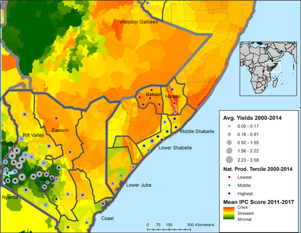
Figure 1. Average maize yields from 2000 to 2014 (dots) and IPC (International Phase Classification) scores from 2011 to 2017. Areas with circles are districts where we make our forecasts. Colors inside the circles show which production tercile (nationally) a district falls in (lowest, middle, or highest). The colors in the polygons are average International Phase Classification (IPC) scores, the IPC international standard used for ranking food security and famine situations. Maize producing provinces that we examine in the paper are labeled.
Download figure:
Standard image High-resolution imageGrowing season rainfall varies across the region, in terms of totals and season duration (figure 2), and this is an important aspect of climate controls on production. In most of Kenya's cropping areas, planting for the long-rains season typically begins in March. High production areas in western Kenya and high-elevation central Kenya are least limited by rainfall and have at least five to six-month long wet season. While droughts and pluvials can impact production, this region can grow water-intensive rainfed crops and re-plant in seasons with poor early season conditions. In normal climate years, farm management and pests may have comparatively more influence on production. Maize production is more water limited elsewhere in central Kenya and in northern and eastern Kenya. In these areas the long-rains season typically ends in March or June with the cessation of rains and harvest is in late July or August.
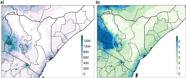
Figure 2. Growing season rainfall in mm (a) and duration in number of months (b). Maps show March to August accumulations to isolate the eastern Horn's long-rains/Gu season. Duration is defined here as the total number of months in this period with greater than 50 mm rainfall. Maps show the median value for 1981–2018 to express a typical season. Data: climate Hazards Center InfraRed Precipitation with Stations.
Download figure:
Standard image High-resolution imageSomalia's long rains (Gu) rainfall season, from April to May or June, is strongly limited by rainfall. The wettest areas in the southwest coastal zone typically receive 400–600 mm of rainfall. Elsewhere rainfall totals are lower and mainly occur during a two-month period. Juba River and Shebelle River flow that originates in Ethiopia's highlands benefits planted riverine areas, such as in Hirraan province and near the coast, but floods can also damage crop fields. Central to eastern Kenya and southwestern Somalia also have a second rainy season between September and December, the short-rains in Kenya and Deyr in Somalia, and there are regions where farmers plant in both seasons.
We analyze the long rains/Gu seasons (in both countries), primarily because the bulk of agricultural productivity occurs during this season. In Kenya the yield data do not differentiate between the long rains and the short-rains season. In Somalia the yield data are cleanly separated between Gu and Deyr seasons (but we only analyze the Gu season). We start our forecasts in March and make a new forecast every month until August. Non-differentiated seasons in the Kenya yield data contributes to uncertainty, particularly for substantive short-rains production areas such as in far eastern Kenya. We explored running forecasts through the end of the year and found that concluding experiments in August allowed for better synthesis of results and retained the value of this analysis. The bulk of early warning for Kenya's long rains season takes place between March and July. After this point even late planted areas are fully established and on-ground assessments of key production areas provide a key information.
3. Methods
Our basic approach is as follows (and shown in figure 3)
- 1.Fit a statistical model between a given EO and observed district-level yields (figure 1) from the period of 1983 to 2000.
- 2.Beginning with 2001, use the fitted model from step 1 and the given EO to predict the end-of-season yields for the current year. Starting in March for Kenya (in April for Somalia), and then for each month until the end of the calendar year, make a prediction using the given EO.
- 3.For the next year (e.g. 2002), update the training data to include the previous year and fit a new model. Make predictions for this year, as in step 2. Repeat the process until the end of the data period (2014), and record the prediction error in each iteration.
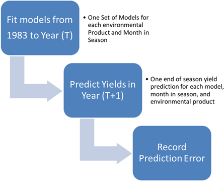
Figure 3. Diagram of approach.
Download figure:
Standard image High-resolution imageThe end result is a set of predicted yields from forecasts made in the months of March to August for every year from 2001 to 2014. The objective is to replicate what prediction error would have been had we been making predictions at the time with the latest available data. We record the prediction error for each month/year it is made and then compare error across spatial units (districts) and calendar months. We use the mean absolute percentage error (MAPE) as our metric of forecast accuracy, and we present the range of MAPE scores across statistical models to evaluate our results. Specifically, the MAPE is:
where yt is an observed value in growing year t and f(t,c) is the forecast of that value at during calendar month c of growing year t. For our purposes, the MAPE in a given district would be the average absolute forecast error (as a percentage of the observed value) of all end-of-season forecasts made from March (or April, in the case of Somalia) of 2001 through August of 2014 (we calculate MAPE score for each calendar month a forecast is made.) We choose the MAPE because it is easy to calculate, intuitive, and scale independent—meaning that forecast accuracy can be compared across grains and volume units. We generate our forecasts from an ensemble of regression models described in the next section.
We use empirical models of maize yields, where yields are a function of an environmental predictor, a time trend, and a set of dummy variables accounting for unobserved factors that vary over space. We fit several flexible model specifications that allow the coefficients on the environmental term to vary across spatial units or across the range of the environmental variable. This modeling framework allows for spatially varying effects not controlled in the environmental variables or in the dummy variables, and also allows for potential nonlinear effects in the response of maize production to extreme environmental conditions (Hansen and Indeje 2004, Schlenker and Roberts 2009, Lobell et al 2011, Davenport et al 2015, 2018). The model specifications we use are shown in equations (1)–(4)


The dependent variable is maize yields (y) (metric tons per hectare) in district (i) at the end of growing year (t). The terms α, γ, δ, and β are all coefficients to be estimated, f() indicates a function, and the model errors are represented by ε. The models are updated each time the model is re-estimated for a given year and calendar month, but the coefficients do not vary over time in a given estimation. Each model incorporates a time trend (Year) to account for unobserved linear changes over time (such as access to agricultural technologies) and a regional fixed effect (District) to account for unobserved factors that vary across space (regional differences in farming practices, policies, and other potential physical effects not accounted for by the EO products). Our key predictors (shown in table 1), are represented by the term ENV and are indexed by district, growing year, and calendar month (c).
We expect coefficients for precipitation, soil moisture, WRSI, and NDVI to have a positive effect on yields, and we expect evaporative demand to have a negative effect. However, the relative size of these effects may vary across regions in ways not accounted for by the fixed effect, and across the range of the variables themselves. Spatially varying and nonlinear effects are accounted for in different ways in models 2–4. Model 2 allows for the effect of the environmental variable to vary across districts. Model 3 fits smooth functions (denoted by f(.)), using a generalized additive model (GAM), across the range of the environmental variables, allowing for the fact that light-to-moderate moisture or heat conditions may not have the same impact on maize yields as extreme moisture or heat. GAMS are widely used in predictive modeling, as they provide a flexible, transparent, and computationally efficient method of accounting for nonlinear relationships in a regression framework. Model 3 allows for smooth coefficients for the environmental variables, while model 4 fits a different smooth term that varies across provinces (p), which are administrative units that encompass districts. We fit both these models (3 and 4) with thin plate regression splines (t.p.r.s) estimated by penalized maximum likelihood using the gam() and s() functions from the mgcv package in R (Wood 2003). The primary advantage of the t.p.r.s. is that a user does not need to specify the knots (transition points between linear pieces), while the estimation procedure leaves the linear components of the fit unchanged (Wood 2003).
We also compare the performance of models that include environmental predictors with those that do not. We use these baseline models to evaluate whether or not the environmental predictors provide any additional information on yield outcomes. Specifically, we evaluate against three baseline models:


The first baseline model (5) includes the first three terms as in (1), an intercept, a time trend, and dummy variables for the district, and fits a panel model (using all districts) as in (1–4). The second (6) and third (7) baseline models are both district-specific time series models. Model (6) uses a district specific time trend, while model (7) uses a lagged, five-year moving average of yields (the mean of yields in years t-1 to t-5). We focus our results on EO products that can perform better on all three baseline models.
4. Results
We first summarize forecast accuracy stratified across high, medium, and low level producers (figures 4 and 5), and then we present the spatial and temporal patterns of forecasts that outperform the baseline models (5–7) described above (figures 6 and 7).
We find that in both countries and across products, forecast accuracy is higher in areas with higher maize yields. This can be seen in figure 4 (yields versus forecast accuracy) which is a plot of forecast error (lower MAPE scores indicate more accurate forecasts) on the y-axis versus average yields (2000–2014) for Kenya and Somalia and each EO product. To add some context for overall food production, districts are colored according to national production tercile (based on production values averaged from 2000 to 2014). There is a strong positive relationship between yield and accuracy in districts with yields around 1 metric ton per hectare or lower in both countries. Accuracy in Somalia is highest (MAPE < 25%) for districts with the nationally highest yields of ∼0.9 to 1 metric tons per hectare. Interestingly, accuracy in Kenya in similar yield-achieving districts is lower than in Somalia, with MAPE scores around 30%–40%.
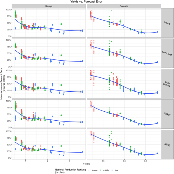
Figure 4 Average Yields versus Forecast Accuracy: this figure plots mean MAPE (mean absolute percent error, y-axis) against average yields from 2000 to 2014 (x-axis) for Kenya (left column) and Somalia (right column). The rows correspond to the EO variables used to make the predictions. Each point represents average forecast error for a given district during a specific calendar month. The blue trend line in each panel plots the relationship between predictive accuracy and average yield size. Colors indicate national production tercile rankings (lowest, middle, and top) based on average production from 2000 to 2014.
Download figure:
Standard image High-resolution imageFigure 5 shows predictive accuracy (y-axis) for each district over the course of the calendar year (x-axis). As in figure 4, the data are grouped by their national production ranking (top panel is lowest tercile; bottom is highest tercile). We find that forecasts tend to be most accurate in high production districts, which is consistent with the increased accuracy for higher yield areas9 . Higher producing areas in Kenya (mostly in the Rift Valley and Western regions) have an average error rate of around 25%, while in Somalia, errors in the higher-producing regions (Middle and Lower Shabelle) are around 20%. Average forecast accuracy for middle (middle row) and lowest (top row) production areas is about 40% in Kenya and 50% in Somalia. The error rate for mid-level production areas in Kenya is driven up by one outlier in the Eastern Region (green line, middle row of Kenya diagram) with most middle production areas being in the 30%–35% range. Figure 5 shows some changes in accuracy through the season and differences across products; however, these are much more muted than spatial variations. These spatial and inter-product variations are examined more in depth below.
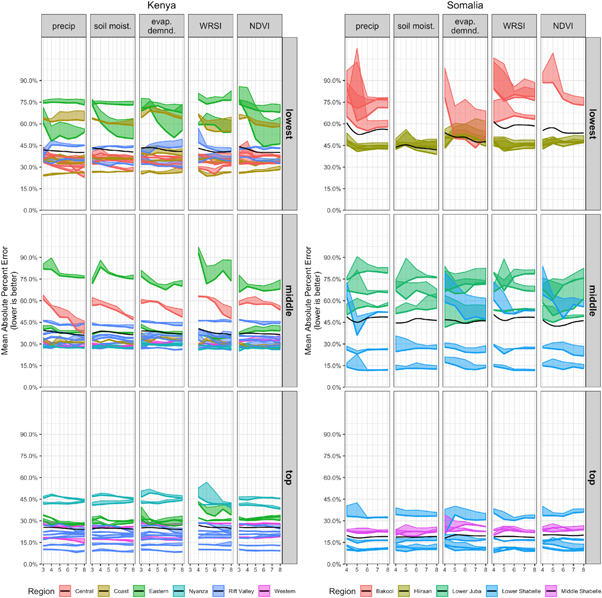
Figure 5 Prediction error (y-axis) over calendar months (x-axis). The solid colored lines indicate the minimum MAPE score (across all model specifications) while the shaded area shows the range of MAPE scores across model specifications. The solid black line plots the average MAPE score for each production tercile. The columns show the EO product used to make the forecast, and the rows group the districts into the top, middle, and lowest producers (according to National production tercile). The left plot is for Kenya and the right panel is for Somalia; the colors represent geographic regions within each country (as shown in figure 1).
Download figure:
Standard image High-resolution imageWe expect forecast accuracy to improve in models that use EO products versus those that do not. Figure S2 compares forecast accuracy of models that use EO products versus the district specific baseline models in equations (5)–(7). Specifically, the plot shows difference in MAPE scores (lower is better) between a model that uses a given EO product and the best performing baseline model for a given district. In Kenya, panel models with environmental predictors generally outperform baseline models in most of the middle-producing regions, likely because they have consistent production and tend to be rainfed. In top-producing regions, most but not all products outperform the baseline models. However, there are notable exceptions, especially in the high-producing, predominantly irrigated areas (mostly in western Kenya) where we cannot capture dynamics associated with irrigation and other more advanced technologies that may be better captured by a district-specific model. In the lowest-producing regions, the results are more mixed, where most products have marginal increases over the baseline but where some do much better or much worse. In Somalia, where even higher-level producers are primarily rainfed, most EO product models do outperform the baseline in the high and low producing districts.
In figure 6, we further explore the relationship between predictive accuracy, EO product, maize production, and how this relationship varies depending on when in the calendar year the forecast is made. In order to focus on the most useful products and identify areas and times of the year where accurate forecasts are possible, we have removed any district/month/product combinations where the EO-based forecasts are less accurate than the forecasts from baseline models (i.e. where the EO-based MAPE score exceeds the MAPE score from any of the baselines models (5–7)).

Figure 6. The y-axis shows the percent of districts where a given product provides the most accurate prediction for end-of-season yields. The x-axis shows the month when the prediction is made. The colors represent the lowest (red), middle (green), and top (blue) terciles of production based on national ranking. Results for Kenya are shown in the left column, results for Somalia are shown in the right column, and the rows correspond to the various products.
Download figure:
Standard image High-resolution imageFocusing first on Kenya (figure 6, left column), we see that for yield forecasts made in March, precipitation (top row), soil moisture (second row), evaporative demand (third row), and NDVI (bottom row) are the best products for approximately 55% of the districts. Of these districts, forecasts made for middle and top production areas (green and blue areas in figure 6) are best when they use soil moisture, evaporative demand, and/or NDVI products. However, in Kenya the more recent MODIS-AQUA based NDVI products (see figure S4) may be better than soil moisture for early season prediction of middle-tier producers.
For top-level producers (blue area in figure 6), soil moisture, NDVI, and evaporative demand are the best products for most districts through May, while evaporative demand is best in June, July, and August. For most middle-producing districts (green), the best products are NDVI in April and WRSI in May and June. Overall, we find that NDVI is generally better suited for mid and top-level producers than for low level producers. This finding is highlighted when comparing NDVI results between the GIMMS (figure 6) and MODIS (figure S4) NDVI products, where in most calendar months, both NDVI products provide the most accurate forecasts for a higher percentage of mid and high level producing districts than for low level producing districts.
For low-level producers, WRSI and precipitation are best in April through June. After June, the long-rains will have mainly concluded in eastern Kenya, and products tend to change minimally in those areas after July. Figure 6 indicates that for middle-to-low producers, many of which fall into this category, late-season forecasts can be informed by WRSI, NDVI, or cumulative precipitation. The top-producer locations are more likely to have continued changes in the predictors through August, and for these, evaporative demand and precipitation appear most useful10 .
In Somalia (figure 6 right panel), where rainfed agricultural dominates, soil moisture and precipitation are the best products for most districts, especially in early months. In the mid-to-late season, soil moisture, evaporative demand, and WRSI are the best products, with soil moisture generally being best among low-level producers, while evaporative demand and WRSI perform best among middle and top-level producers. In contrast to Kenya, the NDVI products are less useful, especially for lower-level producers.
We further explore the spatial patterns in these results in figure 7. As with the previous plot, in this figure, we only show districts where, for a given month, a product can make a forecast that is better than all the baseline models (5–7). Areas marked as 'none' areas, are areas where no product can outperform the baseline model.
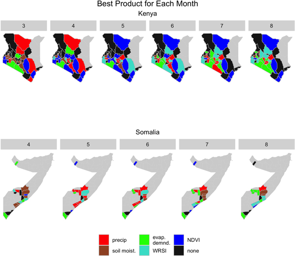
Figure 7. Maps showing the best product for each month. Panels indicate months starting with approximate planting month through the end of the calendar year. The colors indicate which product is best for a given district in a given month. The 'none' category indicates that no product was able perform better than three baseline models. Gray indicates areas where either no (or minimal) maize planting occurs or where long-term data are unavailable.
Download figure:
Standard image High-resolution image
In Kenya, there are some districts where one product remains the best predictor throughout the season, while other regions are more dynamic, switching between products. The 'theoretical ideal', where the results match what we would expect, is in northern central Kenya: low-producing, food insecure region where crop production is predominantly rainfed. Here we see that precipitation is best in the early months (March–April) during the planting and emergence stages, while NDVI (indicative of plant productivity) is better for the remainder of the season. By contrast, in the higher-producing areas of western and northwestern Kenya, none of the EO-based models are more accurate than baseline models. This is probably due to the fact that production in these areas is generally less limited by climatic factors and because EO products cannot capture influences from irrigation, fertilizer, and other characteristics common to commercial agriculture. However, EO products are more skillful than the baseline models over the medium-to-high-level producing, but more climatically limited, regions of southwestern Kenya. In general, evaporative demand and NDVI products are most skillful in those regions.
In Somalia, we see the dominance of the precipitation product (red) and soil moisture in the early months with evaporative demand (green) and WRSI (light blue) providing higher accuracy later in the season. Still, precipitation and soil moisture produce the best estimates during most of the year in the highly food insecure regions of Hiraan and Middle Shabelle (see figure 1) in central Somalia. Somalia in general has more rainfed regions and less commercial agriculture, and the data are better defined by seasons, so we generally see fewer districts (compared with Kenya) where the EO products do not outperform the baseline models.
5. Discussion and conclusion
We find that higher-producing areas tend to have more accurate predictions, but that this relationship plateaus in areas with yields averaging more than one metric ton per hectare. We speculate that this is due to more accurate reporting and measurement in key food-producing areas. In addition, the highest-producing regions tend to have the best environmental conditions and agricultural infrastructure, and thus tend to produce more consistent yields across seasons (see figure S1). However, in these same regions, such as western and northwestern Kenya, models that use EO products are not more accurate than than the most accurate of the baseline models. EO products are ideal in regions with relatively consistent production but where climatic factors still provide some limitations on overall yield levels. In general, these are medium-to-high-level producers growing crops outside of the wettest regions. An example of this would be the top-level producers in Somalia, who are predominantly rainfed but still maintain relatively consistent levels of production.
More generally, we find that precipitation tends to be a better predictor of crop yield among the low rainfall regions which are also lowest producers (figures 1 and 2), whereas evaporative demand tends to be a better predictor of crop yields among the high rainfall regions which are typically also the top producers (figures 1 and 2). In the regions with high rainfall such as southwest Kenya, rainfall is greater than evaporative demand and hence the consumptive use of water (which is directly linked to crop yield) is controlled by the available energy. In other words, variability in evaporative demand would determine the variability of consumptive water use, and hence influence crop yield (though this relationship is more difficult to model in irrigated regions, such as western Kenya). On the other hand, in the low rainfall regions (which includes parts of Central and East Kenya and most of Somalia), it is the rainfall which determines the available moisture and has a more direct relationship to crop yields.
Soil moisture-type products also do well in higher-producing regions. We believe that soil moisture performs better in the higher-producing areas because soil moisture carries over between seasons and does not dry out completely as in the drier, lower-producing regions in the north. Lower producing regions, especially in Somalia, are less able to mitigate against mid-season drought, which is better captured by rainfall than soil moisture product, which retains 'memory' of moisture from earlier in the season.
Our results have several implications for food security monitoring and agricultural planning. If the goal is to assess overall national productivity (assuming that transport constraints are not a problem), then moderately accurate forecasts can be made relatively early in the season. For example, supplemental figure S5 shows that by July, forecasts made with environmental products outperform baseline models for about 70% of total national production in Kenya (left panel of S5). In Somalia, using the same criteria (where environmental products outperform baseline models), just over 95% of national production can be predicted as early as May.
There are several ways that these results can be used to enhance decision-making in sub-Saharan Africa. An operational system for EO-based subnational yield forecasts could be integrated with existing food security assessments, for example, by the Famine Early Warning Systems Network (FEWS NET). FEWS NET publishes monthly to bimonthly reports on market prices and key messages for stakeholders about seasonal rainfall performance and food security status for agricultural and pastoral livelihoods. They also deliver information on an ad hoc basis during global price spikes, conflict, or mass-migration (refugee) events. Several of the products we evaluate are already used in FEWS NET formal or informal yield outlooks during the growing season. The results in this paper provide a structure that identifies where and, potentially, when (in the season) each product might be optimal for qualitative or quantitative outlook assessments in Kenya and Somalia. We also identify areas where EO products do not perform better than simple trend or rolling average models. The analysis could also be applied in other countries where comparable yield data are available. Tables and figures listing optimal products by district/month integrated within an existing outlook system, such as the GEOGLAM crop monitor11 , could provide a quantitative complement to the qualitative analyses provided by that program. However, we do not anticipate that these results would inform the more rigorous, but also more data-dependent, crop modeling and forecast systems used in more developed regions in North America, Europe, and Australia.
Going forward, we believe that these results could be used as starting values in a machine-learning program designed specifically for dynamically updated forecasts. Such a system might focus more on classification, such as predicting very low yields, rather than the specific point forecasts we focus on in this paper. Ultimately, we hope that these results could provide the foundation for a formal decision support system that uses end-of-season yield estimates as a component and is hosted by an East African institution.
Prior to development of an operational system, however, there are several limitations to this study that can be addressed in subsequent research. Many more recent EO products are available with higher temporal resolution. Knowledge of precise planting dates paired with EO measures of sub-monthly shocks would likely allow for increased accuracy by more precisely pairing sub-seasonal metrics with crop phenology. In this paper we mostly use a fairly crude set of metrics, cumulative sums, means, or maximum values through the season. Exploring rolling values, alternative measures of aggregation, or empirically based seasonal weights all have the potential to increase forecast accuracy. We could also fully evaluate the degree to which products with a finer spatial resolution do or do not contribute to forecast accuracy when aggregated to the district level. Other avenues for expanding this study include comparing panel and univariate time series approaches, and the sensitivity of forecast accuracy to varying seasonal start and end dates. In addition, forecast accuracy would probably increase when using multiple EO predictors if they contribute unique information pertaining to, for example, early versus late stages of plant phenology. Information from our modeling experiments could guide the development of promising, physically based multivariate models for administrative zones in Kenya, Somalia, and elsewhere.
Data availability statement
The maize yield data set comes from reports produced by the Kenyan Ministry of Agriculture, Livestock and Fisheries and the FAO Food Security and Nutrition Analysis Unit (FSNAU) for Somalia. The data have been collated by the FEWS NET Data warehouse project. There are restrictions to the usability of the yield data, which were used under special permission and are not publicly available. The data that support the findings of this study are available from the corresponding author upon reasonable request. The data are not publicly available for legal and/or ethical reasons.
Footnotes
- 6
After applying the crop mask and filtering for districts with consistent yield data, we analyzed 36 districts in Kenya and 20 districts in Somalia. Supplemental table S1 lists the total number of districts analyzed by country and region.
- 7
While there are newer products available over a finer spatial and temporal resolution, these are not necessarily ideal for forecasting district level end-of-season yield outcomes. The advantage of fine spatial resolutions might be reduced when products must be aggregated over districts to match the spatial support of the yield data, and the finer temporal resolution products are most useful if exacting planting dates are known so that seasonal patterns can matched more closely with crop phenology.
- 8
With the MODIS products, we fit models to the period 2003–2008 (versus 1983-2000 for the other products), and then conducted 1-step ahead forecasts for the years 2009–2014 (versus 2001–2014). Because the training and evaluation periods were conducted over a different period as with the other products, comparisons should be made with caution.
- 9
While district-level production and yields are correlated, there is a not a direct one-to-one relationship. Some districts have high yields but do not make substantial contributions to national production because the cropped area is small. Conversely large districts with lots of cropped area may have more limited yields due to climate controls and less access to agricultural technologies and infrastructure. For example, when ranking 10 year averages of production and yield, Elgeyo-Marakwet in the Rift Valley is ranked 5th in yields but 14th in production. Conversely, Machakos in Eastern Kenya, ranks 11th in production but 32nd in yields.
- 10
Supplemental figure S3 presents the same results but also includes a model that uses separate coefficients for precipitation and evaporative demand (two independent products that separately account for water supply and demand). June and July are the best months when using precipitation and ET0 in the same model (the row labeled 'P + E' in fig. S3). Supplemental figure S4 presents the same results but also includes results for the more recent MODIS-AQUA based NDVI and EVI products.
- 11