

Abstract
The European summer of 1816 has often been referred to as a 'year without a summer' due to anomalously cold conditions and unusual wetness, which led to widespread famines and agricultural failures. The cause has often been assumed to be the eruption of Mount Tambora in April 1815, however this link has not, until now, been proven. Here we apply state-of-the-art event attribution methods to quantify the contribution by the eruption and random weather variability to this extreme European summer climate anomaly. By selecting analogue summers that have similar sea-level-pressure patterns to that observed in 1816 from both observations and unperturbed climate model simulations, we show that the circulation state can reproduce the precipitation anomaly without external forcing, but can explain only about a quarter of the anomalously cold conditions. We find that in climate models, including the forcing by the Tambora eruption makes the European cold anomaly up to 100 times more likely, while the precipitation anomaly became 1.5–3 times as likely, attributing a large fraction of the observed anomalies to the volcanic forcing. Our study thus demonstrates how linking regional climate anomalies to large-scale circulation is necessary to quantitatively interpret and attribute post-eruption variability.
Export citation and abstract BibTeX RIS

Original content from this work may be used under the terms of the Creative Commons Attribution 3.0 licence. Any further distribution of this work must maintain attribution to the author(s) and the title of the work, journal citation and DOI.
1. Introduction
Global temperatures were exceptionally low in 1816, and it was probably the coldest year for at least the last 250 years (Crowley et al 2014). One of the most noticeable impacts was felt in Central and Western Europe, which had a particularly cold and wet summer (Luterbacher and Pfister 2015, Brönnimann and Krämer 2016) with increases in cloud cover (Auchmann et al 2012). The summer was so extreme that in Europe and North America it has often been described as a 'year without a summer'. The anomalous climate led to considerable societal effects with a greatly reduced harvest contributing to the 'last great subsistence crisis in the Western World' (Post 1977).
The eruption of Mount Tambora in Indonesia (8 °S, 115 °E) in April 1815 was among the most explosive of the last millennium and had an enormous impact locally, devastating the island of Sumbawa. The eruption injected a huge amount of SO2 into the stratosphere (Oppenheimer 2003), which would have quickly spread across the globe, oxidising to form sulphate aerosols. The effect of volcanic aerosols on the climate have been extensively studied and they have been shown to reduce net shortwave radiation causing widespread long-lasting surface cooling (Robock 2000, Fasullo et al 2017). In addition large volcanic eruptions have been shown to lead to a reduction in global precipitation (Iles et al 2013), a shift of the Inter Tropical Convergence Zone away from the hemisphere of maximum forcing (which can have a considerable effect on monsoon rainfall; Stevenson et al 2016) and can wetten some dry regions (Iles and Hegerl 2015). They also induce dynamic changes in the large-scale circulation of both ocean and atmosphere (Zanchettin 2017). The eruption of Mount Tambora is therefore very likely to have had a profound impact on a global scale (Raible et al 2016), causing widespread extreme climate fluctuations throughout the world in its aftermath and the following years.
A link between the Mount Tambora eruption and the year without a summer was made as early as 1913 by Humphreys (1913) and the 1816 year without a summer is now typically attributed to the eruption of Mount Tambora (see Raible et al 2016 and references therein). However, in addition to the volcanic effects other studies have also suggested a major role for internal climate variability, not linked to the volcanic activity (Auchmann et al 2012, Brönnimann and Krämer 2016) as well as a possible contribution from a period of low solar variability, the Dalton minimum (Anet et al 2014). Event attribution analyses are used to estimate how much human influences have affected the probability for recent extreme events (see e.g. National Academies of Sciences, Engineering and Medicine (2016), Stott et al 2016). Here we use early instrumental data (Casty et al 2007, Küttel et al 2010) combined with new climate simulations from two different models to conduct, for the first time, an event attribution analysis in order to determine if and by how much the volcanic forcing has affected the probability of cold and wet conditions in this 'year without a summer'. We choose to focus our analysis on Central Europe (here and throughout the paper defined as latitude 40° to 55 °N; longitude 5 °W to 20 °E) where the most extreme climate anomalies occurred.
2. Data
2.1. Climate reconstruction data
Surface air temperature and precipitation are taken from the gridded datasets of Casty et al (2007), which have a resolution of 0.5° × 0.5°. These datasets are calculated using Principal Component regression using transfer functions calculated during periods where information is available from both station data and the gridded climate information used for calibration (Mitchell and Jones 2005). For the early 19th century, more stations are available from central Europe (see figure S2(b) and (c) available online at stacks.iop.org/ERL/14/094019/mmedia) leading to better reconstructions in this area. To remove the effects of anthropogenic warming in the datasets we detrend the temperature observations using a second order polynomial fitted to Central Euopean mean temperature (figure S1).
Sea-level pressure (SLP) gridded datasets are taken from Küttel et al (2010). The gridded product uses station SLP data and wind direction and wind strength derived from ship logbooks and constructs 5° × 5° gridded information from a multivariate principal component regression using the dataset HadSLP2 (Allan and Ansell (2006)) as a target. In the early 19th century reconstruction skill is highest for winter. For summer (the season of interest in this work) skill is much higher over continental Europe than over the Atlantic. And for the Atlantic skill is higher (and consistently better than climatology) in the northern part (50°–70 °N) than the south (20°–45 °N) where the reconstruction has no more skill than climatology.
All climate reconstruction results are shown as anomalies from the mean of the period 1781–2000
2.2. Atmosphere-ocean general circulation model data
2.2.1. MPI-ESM1.2
We use version1.2 of the Max Planck Institute for Meteorology Earth System Model (MPI-ESM1.2, Mauritsen et al 2019), as developed for use in the Coupled Model Intercomparison Project 6 (Eyring et al 2016). All simulations have been performed with the low resolution version of the MPI-ESM1.2 with a horizontal resolution of T63 (∼200 km) and 47 vertical layers in the atmosphere and a horizontal resolution of GR15 (∼150 km) and 40 vertical levels in the ocean. We make use of a 1300 year long-time piControl run (constant forcing at year 1850 pre-industrial levels) and have performed a series of early 19th century simulations starting from different initial dates from the piControl simulation with different volcanic only forcing estimates (as described in Zanchettin et al 2019). These are based on the evolv2k forcing reconstructions (Toohey and Sigl 2017) and have been compiled with the Easy Volcanic Aerosol (EVA) forcing generator (Toohey et al 2016). We use three forcing volcanic time series: a central (Best), high-end and low-end estimate, corresponding to the central estimate plus/minus 2 times the 1σ sulfur emission uncertainty (hereafter High and Low). 90 ensemble members are available in total for the summer of 1816, 30 for each forcing estimate. We focus in the paper on results using the best forcing estimate, but report all results in some figures and in the supplementary information. The aerosol optical depth for the three volcanic forcings is shown in the supplementary information (figure S3).
2.2.2. HadCM3
We use model simulations from the coupled atmosphere–ocean model HadCM3 (Gordon et al 2000, Pope et al 2000). The atmosphere has a horizontal resolution of 3.75° × 2.5° in longitude and latitude with 19 vertical levels. The ocean model has a resolution of 1.25° × 1.25° with 20 levels. The model simulations used are a 1200 year long piControl simulation (constant forcing at year 850 pre-industrial levels, as described in Schurer et al 2013) and 50 simulations with volcanic forcing. The volcanic ensemble members have been started using different initial conditions taken from the piControl control simulation and run using only volcanic forcing, using the aerosol optical depth estimates from Crowley and Unterman (2012). The aerosol optical depth for the volcanic forcing is shown in the supplementary information (figure S3). The simulations start in December 1814 and run for two years, encompassing the Tambora eruption in April 1815 and the Summer of 1816.
For both models all results are shown as anomalies from the climatology of their respective control simulation.
3. Methods
A circulation analogues method selects periods that display a similar surface or mid-troposheric flow pattern to an event that has been pre-selected (Jézéquel et al 2018). Here we use it to select summers which have similar SLP patterns to that observed in 1816. We select analogues based on the domain 40 °W to 25° E and 40 °N to 70 °N, which is chosen to concentrate on continental Europe and the North Atlantic which are the regions with the most reconstruction skill (see data section). As in Yiou (2014), the analogues are selected to be those with the smallest area-weighted root mean square error (RMSE), calculated by summing over the difference between the SLP in each summer with the target SLP field for all of the grid boxes within the domain. We show results for the mean of those analogues which have RMSE values less than a pre-defined threshold. For the main results this threshold is calculated so that for the instrumental observations 10 analogues are selected. The equivalent number of analogues for the models without volcanic eruptions is 61 while only 2 analogues for the models with volcanic eruption met this criterion (due to a smaller number of sample years to choose from). Alternative threshold values yielding 5 and 20 observational analogues were also analysed and the results were found to be insensitive to this choice.
In order to quantify how the volcanic forcing changes the likelihood that the summer after the eruption is as cold and wet as that observed in the 1816, we calculate return times based on model simulations, where the return time is the inverse of the probability of an event occurring per year, and gives the likelihood of the event recurring within a certain time interval. Return times are calculated for both the model simulations forced by the volcanic eruption and the piControl simulations which do not contain volcanic eruptions. An increase in likelihood of an event can be calculated by comparing the return times with and without volcanic eruptions.
To calculate the return times for a specific event, in this case the summer of 1816, a Gaussian distribution was fitted to the modelled values for mean summer European temperature, precipitation and SLP and the return time calculated from the point where the distribution crosses the event threshold. An uncertainty estimate is calculated using a non-parametric bootstrap analysis, in which 10 000 new model samples are created by randomly selecting from the original model sample, a Gaussian distribution is then fitted and a return-time is calculated for each. A 5%–95% range can be calculated from the distribution formed from the 10 000 return time values. An increase in likelihood of the event (the risk ratio) is then calculated from the ratio of the return times for the two different scenarios and the uncertainty in this is calculated using the 10 000 pairs from the the two return time distributions. To sample the sensitivity to the choice of distributions we also calculate return times with gamma and skew-normal distributions with results shown in the supplementary information (figures S10 and S11).
4. Results and discussion
The year 1816 was unusually cold in large parts of Europe and, in particular, in Central Europe, with every season showing negative temperature anomalies (figure 1). However, it was in summer that the largest temperature anomalies occurred, with the coldest recorded European mean summer temperature in the 235-year long (1766–2000) instrumental-based dataset (Casty et al 2007), and the coldest in the Central England Temperature series (Parker et al 1992) during this period (although 1695 and 1725 were colder). This summer was also anomalously wet in central Europe, although not as extreme, with 19 wetter summers recorded between 1766 and 2000. This is consistent with the England and Wales precipitation series (Wigley et al 1984, Alexander and Jones 2000) in which the summer of 1816 is the 22nd wettest for the same period. These findings are supported by other instrumental datasets and a reanalysis product (see figure S2) which also show that the summer of 1816 was very cold and wet in Europe (Pauling et al 2006, Luterbacher et al 2016, Anchukaitis et al 2017, Franke et al 2017). Climate anomalies are most prominent in summer when the direct response to radiative forcing largely determines climate variability, whereas in other seasons, in particular winter, forced responses are more strongly mediated by strong dynamically induced variability (Zanchettin et al 2019). The temperature and precipitation in the first and second post-eruption year after nine other volcanic eruptions between 1781 and 2000 display on average only a slight decrease in summer temperature (see figure 1), although this is more notable if a longer period with more volcanic eruptions are analysed (see figure S8 and Fischer et al 2007). These eruptions are all smaller than Mount Tambora (Toohey and Sigl 2017), so it is unsurprising that the climatic impact of these eruptions is not as large. They also occurred in different months of the year so should be expected to have different impacts on seasonal means (Stevenson et al 2017).
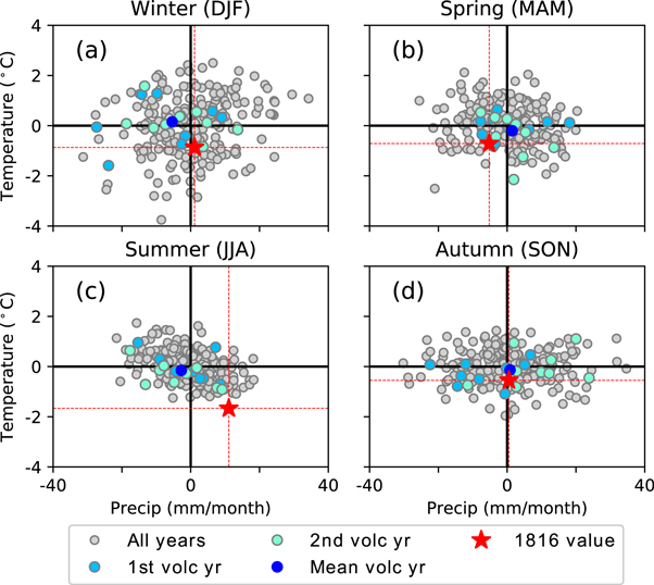
Figure 1. Observed Central European climate anomalies in the, year without a summer, (latitude 40° to 55 °N; longitude 5 °W to 20 °E; 1781–2000) compared to other volcanic and non-volcanic years. Seasonal temperature (vertical axis) and precipitation anomalies (horizontal axis) relative to the long-term mean. Values for 1816 are shown by red star and red dashed lines. Other volcanic years are shown as blue circles (year after eruption light blue, second year after eruption aquamarine, mean of first two years following all eruptions dark blue), other non-volcanic years as grey circles. Data from Casty et al (2007); global warming subtracted (see methods).
Download figure:
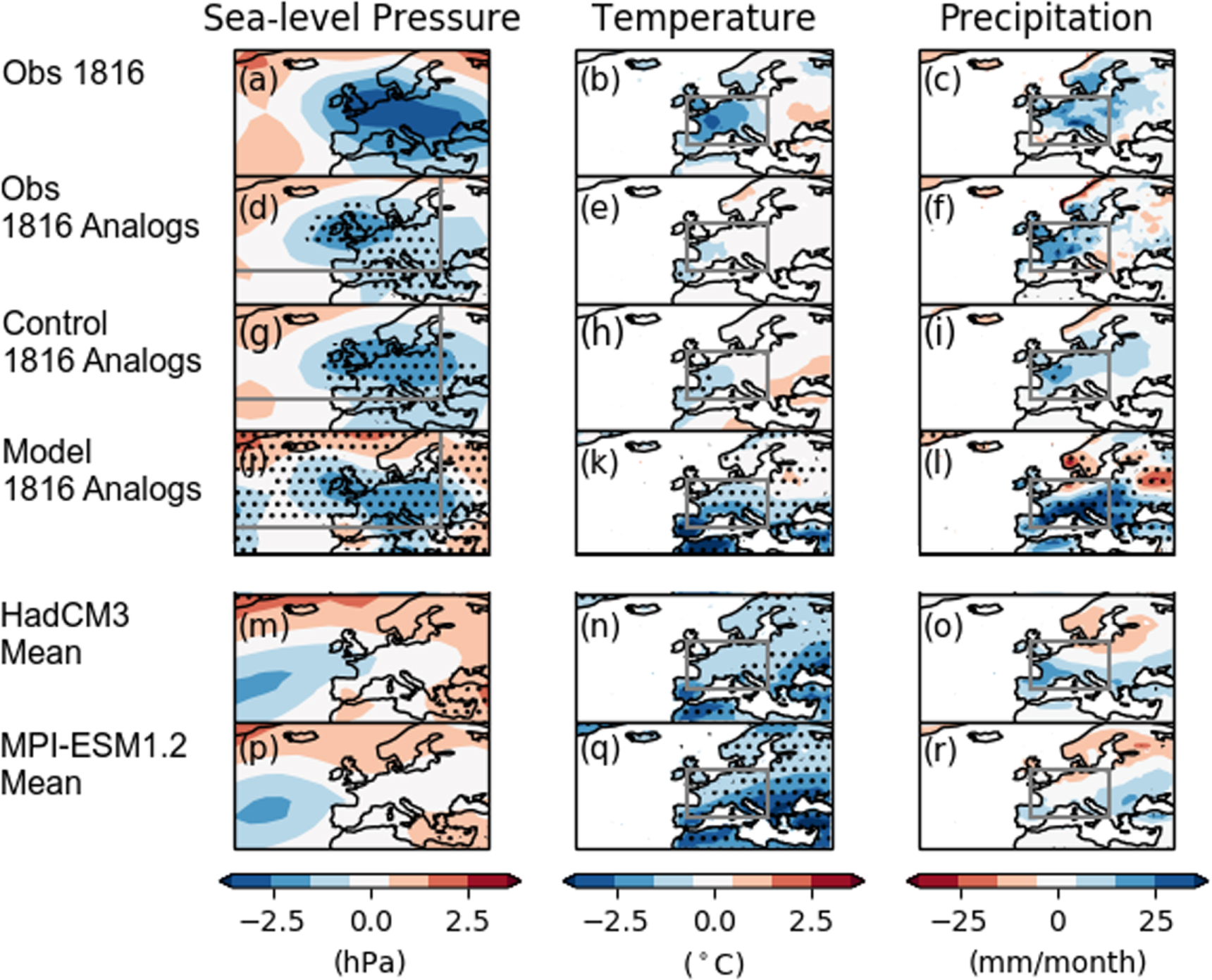
Standard image High-resolution imageSpatially extrapolated instrumental datasets show that the summer of 1816 was characterised by an anomalous low pressure system centred over Northern Europe (figure 2(a)), with Central European mean values among the most extreme since at least 1780 (figure S1d and Luterbacher et al 2002, Küttel et al 2010, Franke et al 2017). The anomalously cold and wet conditions are accordingly centred over western and central Europe and southern Scandinavia. Eastern Europe and western Russia did not experience large temperature or precipitation anomalies. To determine the role that this anomalous atmospheric circulation played in the summer of 1816, the SLP patterns in all other summers are compared to that observed in 1816 with the 10 most similar years in the record used as analogues for the event itself (see method section). Analogue patterns can be found which have SLP patterns similar to that observed (figure 2(d)); hence, they show a low-pressure anomaly over Central and Northern Europe. The analogue years have similar high precipitation anomalies over central Europe as in 1816 (figure 3(a)). They also account for the spatial pattern of rainfall (compare figure 2(f) with figure 2(c)). However, the analogue years only show a slight decrease in temperature (an average of −0.4 °C), much less than that observed in 1816 (−1.7 °C) (figures 2(e) and 3(a)), explaining approximately a quarter of the cooling. These results are supported by analyses of unperturbed piControl model simulations, (which do not include volcanic forcing) (figures 2(g)–(i) and figure 3(b)), which also show that the SLP pattern, even with no anomalous forcing, is sufficient to explain the reconstructed precipitation but not the cold temperatures. Model results also show a remarkable agreement in the variability between the unforced model simulations and observed variability in both temperature and precipitation (figure 3(b)), which increases confidence that the climate simulations can adequately represent European summer climate.

Figure 2. Observed and simulated spatial patterns for the summer of 1816: sea level pressure (left), temperature (middle) and precipitation (right) relative to 1781–2000 mean. Top row, observed summer climate from Casty et al (2007) and Küttel et al (2010). Second row, mean of 5 analogues from observations with long-term warming removed (see methods). Third row, mean of best 27 analogues from pre-industrial control simulations. Fourth row, mean of the best 2 analogues from simulations of summer 1816 which include the Tambora eruption. Fifth and sixth row mean of all 50 HadCM3 and 30 MPI-ESM1.2 simulations of 1816 summer which include the Tambora eruption for the summer of 1816. The stipples show 90% agreement of sign. Box in the left panels—region over which analogues are calculated. Box in centre and right panels—area spatial means are calculated over.
Download figure:
Standard image High-resolution image
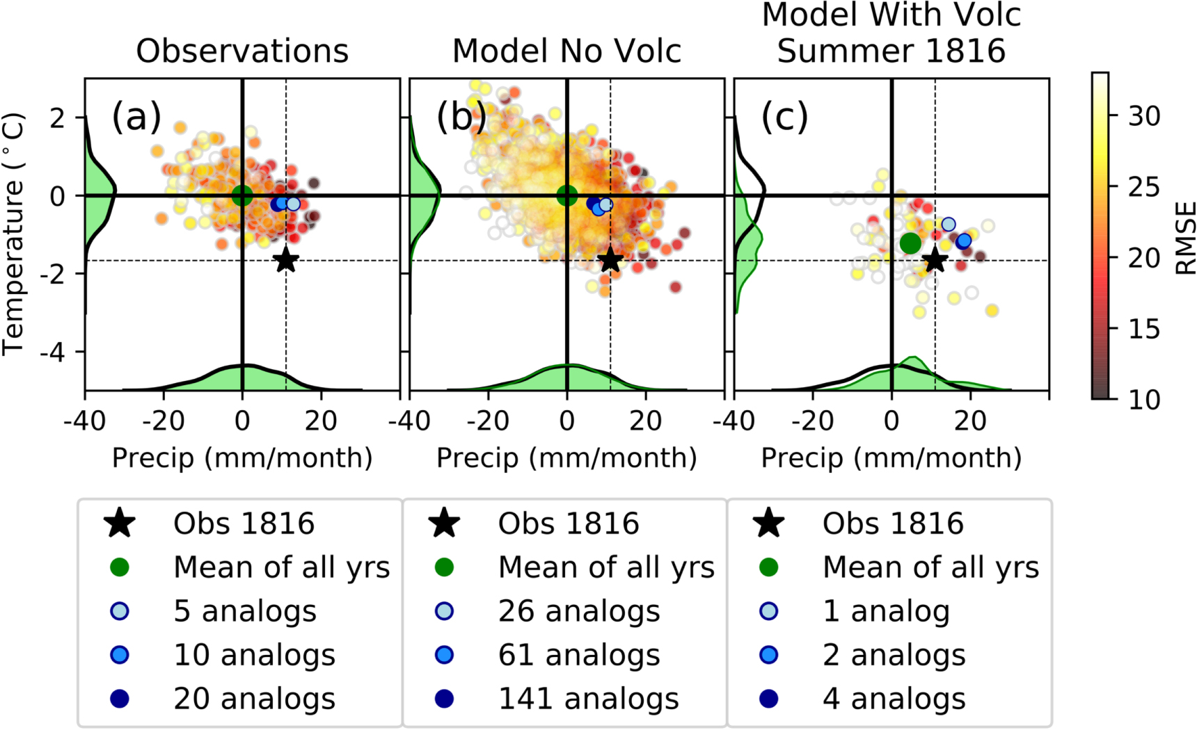
Figure 3. The effects of volcanic forcing and analogue sea level pressure patterns on observed and simulated temperature and precipitation anomalies in Central European summer. (a) Observations and (b) unforced control simulations (MPI-ESM1.2- & HadCM3) with anomalies from the long term mean, (c) model simulations (MPI-ESM1.2- & HadCM3) driven with the Tambora eruption forcing with anomalies from the control mean. Big green circle is the mean of all years. Big blue circle is the mean of the best analogues, where the number of analogues used is given in the legend (see method section). Colour of smaller circles dependent on closeness of observations and simulations to observed SLP pattern determined by RMSE. Black star and black dashed lines—actual observed values in the summer of 1816. Distributions on x and y-axis show observation/model spread where the black distribution in all panels shows observation spread, green shading shows the spread of results in each panel.
Download figure:
Standard image High-resolution imageSimulations of 1816 using two climate models (MPI-ESM1.2 and HadCM3—see data section) that include the Mount Tambora eruption show that the volcanic forcing is likely to have caused considerable cooling throughout Europe (figure 3(c)). Although there is a wide distribution of values for the summer of 1816 (which reflects the large role that internal variability plays in any specific year) there is a clear offset in the distribution with the change in regional mean found to be highly significant in both models (p < 0.001). The mean of all the HadCM3 ensemble members shows slightly less cooling than observed in 1816 (figure S4f) but the ensemble spread is consistent with the observed value. We use three ensembles with MPI-ESM1.2 forced by a low, best and high estimate of what the forcing caused by the Mount Tambora eruption could have been (see data section). We focus largely on the central, best forcing estimate of the Mount Tambora eruption (but results for all three cases are shown in the supplement; figure S4). The MPI-ESM2.1 simulations forced with the lower estimate of the Mount Tambora eruption exhibit considerably less cooling than those with the high estimate of the forcing (figure S4(c) and (e)) showing that summer cooling is very dependent on the forcing (Zanchettin et al 2019). The mean of the experiments with the 'best' estimate of the volcanic forcing is most consistent with the observations, although all ensembles encompass the observed value. Given that we have found a small contribution to the cooling in this region from atmospheric circulation (figure 2) which is not included in the ensemble mean, it is possible that the lower estimate of forcing would actually be the most consistent, if this were included. Indeed, a better agreement between the simulations with the low forcing and reconstructions of summer temperatures was found previously by Zanchettin et al (2019) based on a much wider European mean, for which the dynamical contribution would be expected to be reduced.
There is also a slight increase in average European mean precipitation (which is significant only in HadCM3). This is consistent with a number of other model studies which have also found an increase in precipitation in south-central European summer following volcanic eruptions (Iles et al 2013, Kandlbauer et al 2013, Wegmann et al 2014), and which is broadly consistent with the average observed response following 10 different eruptions (see Fischer et al 2007 and figure S9). The effect of forcing uncertainty (as expressed between the three MPI ensembles) on precipitation is not as strong, nor is the effect on the SLP pattern (not shown). Wegmann et al (2014) linked this increase in precipitation to a southward shift of the North Atlantic jet caused by a weaker African monsoon. Our results support their conclusions, also showing drying of the North African monsoon and similar changes in North Atlantic atmospheric circulation (see figure 2 and supplementary figure S4). Following the eruption of Mount Tambora the precipitation anomaly is instead centred on central Europe so we now quantify if there is evidence the eruption enhanced the probability of increased wetness in this region.
Neither of the SLP anomaly patterns for the year 1816 in the climate model simulations compares well visually with that observed (compare figure 2(a) with figures 2(m) and (p)). The lack of similarity is confirmed by an analysis of the RMSE between the two sets of patterns (figure S5) which does not show any reduction from the RMSE beyond what is expected from internal variability alone. Analogues do exist (figures 2(j)–(l)), however among the volcanically-forced model simulations, which are characterised by a low pressure over Northern Europe and lead to both cold and wet conditions very similar to those observed (figure 3(c)). Therefore, although there is no evidence that the volcanic eruption has made the observed pressure pattern more likely, it does not prevent conditions similar to that observed either.
By creating a composite pattern over all summers which have Central European precipitation anomalies greater than that observed in 1816, it becomes evident that the most significant feature in all cases, both in observations and models (with and without volcanic forcing), is a low pressure anomaly centre over Central and Northern Europe (figure S7). This corresponds to the major circulation feature associated with the summer of 1816 (figure 2(a)) and coincides with the region with the most reliable instrumental data (see Küttel et al 2010 and data section). Consequently, we assume that while the area that we are using to determine the analogues is relatively large the most important region for increased European rainfall is confined to Central and Northern Europe.
The volcanic forcing in the HadCM3 models increases the likelihood of a low pressure over this area by a factor of about 2.5, although whether this change is significant (p < 0.05) depends on the distribution used to fit to the data (see supplementary figure 11). Conversely, the uncertainty in MPI-ESM1.2 results is too large to reach a firm conclusion regarding changes in likelihood (figure 4(e) and table 1). So, although the Mount Tambora eruption may not have increased the probability of the observed large-scale pressure pattern over Europe and the North Atlantic there is some evidence that it has increased the occurrence of the most important feature for extreme European rainfall, namely very low SLP over Central Europe in at least one of the models analysed here. This is consistent with an atmospheric reanalysis study (Brohan et al 2016) which found that including volcanic aerosols improves the consistency, at European instrumental sites, of both temperature and SLP.

Figure 4. Return times plots for the climate of the summer in 1816. The points (coloured circles for experiments with Tambora eruption, green crosses for experiments without) represent return times for events (a) with lower temperatures, (b) higher precipitation and (c) with a lower SLP than the observed values for Central Europe, shown by the horizontal red dotted line. The shading represents the 5%–95% uncertainty calculated by a non-parametric bootstrap analysis. The thin lines show a Gaussian fit to the data. Return time with 5%–95% uncertainty for the 1816 event in each model experiment, is shown by the coloured horizontal line at the bottom (see methods). SLP return times are calculated for the region: 45° to 55 °N, 5 °W to 20 °E. Temperature and precipitation for the region: 40° to 55 °N, 5 °W to 20 °E, as before. All anomalies are calculated relative to the long term mean of the piControl simulations.
Download figure:
Standard image High-resolution image
Table 1. Return times for the summer of 1816 - Return times (in years) and the increase in risk ratio (probability with eruption, relative to without eruption) for different model experiments. 5%–95% uncertainty ranges given in brackets, risk ratio results significant at 5% level are indicated by an asterisk. For temperature three values are given for the MPI-ESM1.2 experiments corresponding to low, best and high volcanic forcings, for precipitation and SLP just the combined values from the three MPI-ESM1.2 experiments are reported.
| Name of Experiment | Return time (years) | Risk ratio | ||||
|---|---|---|---|---|---|---|
| Temperature | ||||||
| HadCM3 No Volc | 855 (603–1256) | |||||
| HadCM3 With Volc | 8.6 (6.0–15.3) | 101* (50–169) | ||||
| MPI-ESM1.2 No Volc | 57 (46–72) | |||||
| MPI-ESM1.2 With Volc | 4.4 (3.1–8.4) | 2.0 (1.6–2.6) | 1.3 (1.2–1.5) | 13* (6.6–19) | 29* (20–39) | 44* (35–55) |
| Precipitation | ||||||
| HadCM3 No Volc | 12 (11–14) | 3.3* (2.1–4.5) | ||||
| HadCM3 With Volc | 3.7 (2.9–5.6) | |||||
| MPI-ESM1.2 No Volc | 9.1 (8.2–10) | |||||
| MPI-ESM1.2 With Volc | 5.7 (4.3–8.3) | 1.6* (1.1–2.1) | ||||
| Sea level pressure | ||||||
| HadCM3 No Volc | 74 (59–92) | 2.5* (1.0–4.4) | ||||
| HadCM3 With Volc | 28 (17–69) | |||||
| MPI-ESM1.2 No Volc | 52 (43–63) | |||||
| MPI-ESM1.2 With Volc | 52 (25–177) | 1.0 (0.3–2.1) | ||||
To address the question of how much more likely the eruption of Mount Tambora made the extreme weather experienced during the summer of 1816 in Central Europe we calculate return times with and without the volcanic forcing (see method section). As figure 4 and table 1 show, the eruption increases the likelihood of a temperature anomaly less than −1.7 °C occurring by about 100 times in HadCM3 and approximately 30 times in MPI-ESM1.2 simulations (with the best forcing - with the lowest estimate (5th percentile of lowest MPI forcing) being a factor of 7). Thus, a very rare event without forcing becomes one that is common in the aftermath of the eruption. It is clear from figure 4 that these results are sensitive to both the model used and the adopted forcing estimate, as shown by the considerable spread in the results in the different MPI-ESM1.2 ensembles, again reflecting the key role of forcing strength on the change in probability of a very cold summer. Even though the increase in the likelihood of the observed wet summer is less than for temperature (figures 4(c) and (d)) the volcanic eruption still increases the chances of the event by a factor of about 1.5–3, an increase that is significant at the 5th percentile in the combined MPI ensembles and in HadCM3 (table 1). Return times show some dependency on the statistical distribution chosen to fit to the data (see supplementary figure S11), however the overall results are not particular sensitive and the choice of distribution does not affect the main conclusions.
There is a notable difference in the results from the two climate models used, with the risk ratios calculated for the HadCM3 model being in general larger than those for the MPI-ESM1.2 model. There are several plausible explanation to these model differences. The experimental set-up is likely to play an important role. A different volcanic dataset is used for each model, which results in a more prolonged tropical forcing in the HadCM3 model, that is still large in the summer of 1816 (see supplementary figure S3). Even when the same volcanic forcing is used, models have been found to react differently on both a large scale (see, e.g. Brohan et al 2012, Zanchettin et al 2016) and on a regional scale (see, e.g. Driscoll et al 2012), which could be both due to differences in how a model implements the forcing and how the forcing impacts on atmospheric dynamics. Disentangling these differences will be a key goal of the VolMIP initiative (Zanchettin et al 2016). In addition, it is clear in figure 3 that differences also exist in the return time for the event in the piControl simulations (those without volcanic forcing). Such differences in return time, which reflects differences in the intrinsic climate variability generated by both models, will also impact on the risk ratio. Furthermore, different climatological biases between models are known to exist in this region (see e.g. Pyrina et al 2017), which could be as a result of differences in parameterisation and the resolution of the model.
5. Conclusions
In Central Europe the summer of 1816 was the coldest summer on record and was also quite wet. This study finds that the atmospheric circulation associated with the SLP pattern in the summer of 1816 is estimated to cause only about a quarter of the cold anomaly observed. Including volcanic forcing in climate models can account for the cooling, and is estimated to increase the likelihood of the extremely cold temperatures by up to 100 times. The observed SLP pattern can account for much of the observed anomalously wet conditions, even in the absence of volcanic forcing. However, there is strong evidence that in the model simulations the volcanic eruption increases the chance of such a wet summer over Central Europe by about 1.5–3 times. There is some evidence that the volcanic forcing increases the chances of the low-pressure system centred over Central Europe, which is largely responsible for the wet conditions. However it leaves open the possibility that other mechanism driven by volcanism could also be causing the wetter conditions over Europe, possibly on a sub-monthly scale (see e.g. Brugnara et al 2015).
Although this study relies on reconstructed climate from early instrumental observations, these have been found to agree well with a number of alternative datasets, so are thought to be reliable. We also do not consider solar forced variability explicitly. Since 1816 falls within the Dalton minimum, solar forcing could have made some contribution to the cold temperatures (Anet et al 2014) despite estimated small response on large scales (Schurer et al 2013). Nevertheless, a significant increase in the risk of both the cold and the wet conditions experienced in 1816 is found when volcanic forcing was included in the two model ensembles analysed in this study, and this is by construction independent of the inclusion of any other forcing.
We therefore conclude that the eruption of Mount Tambora has, with high statistical confidence, played a dominant role in causing the observed cold conditions and probably also contributed to the anomalously wet conditions. Without volcanic forcing, it is less likely to have been as wet and highly unlikely to have been as cold. This study demonstrates how linking regional climate anomalies to large-scale circulation is necessary to quantitatively interpret and attribute post-eruption climate variability.
6. Data availability statement
The volcanically forced HadCM3 model data is available from the University of Edinburgh's DataShare: https://doi.org/10.7488/ds/2601. The HadCM3 control simulation is available from the Natural Environment Research Council's Data Repository for Atmospheric Science and Earth Observation: http://data.ceda.ac.uk/badc/euroclim500/data/DRIFT. The gridded climate reconstruction data is available from the World Data Center for Paleoclimatology: https://www.ncdc.noaa.gov/paleo.
Acknowledgments
The work was supported by NERC under the grant PacMedy (NE/P0067521/1) and the ERC-funded project TITAN (EC-320691). C Timmreck acknowledges support from the German federal Ministry of Education (BMBF), research programmes 'MiKlip'(FKZ:01LP1517B), and the European Union project StratoClim (FP7-ENV.2013.6.1–2). DZ acknowledges support by the DAIS‐IRIDE project (VolClim). SB acknowledges funding from the Swiss National Science Foundation (162668) and from the European Research Council under H2020 (Grant PALAEO-RA, 787574). MPI-ESM simulations were performed at the German Climate Computer Center (DKRZ).