

Abstract
More than 90% of the Earth's energy imbalance is stored by the ocean. While previous studies have shown that changes in the ocean warming are detectable and distinct from internal variability of the climate system, an estimate of separate contributions by natural and individual anthropogenic forcings (such as greenhouse gases and aerosols) remains outstanding. Here we investigate anthropogenic and greenhouse-gas contributions to past ocean warming, and estimate their contributions to future sea level rise by the year 2100. By applying detection and attribution framework (regularized optimal fingerprinting), we show that ocean warming in the historical period is detectable and attributable to contributions from the aggregate anthropogenic forcing as well as greenhouse gas forcing alone. We also discuss the role of natural forcing on the ocean volume-averaged temperature and examine the impact of volcanic activity from the three main volcanoes occurring in the historical period 1955–2012. Our results suggest that estimated anthropogenic and greenhouse-gas contributions to ocean warming are consistent with observations, and observationally-constrained future thermosteric sea level rise projections support the central and lower part of the multi-model mean projection range distribution.
Export citation and abstract BibTeX RIS

Original content from this work may be used under the terms of the Creative Commons Attribution 3.0 licence. Any further distribution of this work must maintain attribution to the author(s) and the title of the work, journal citation and DOI.
1. Introduction
The excess energy in the climate system resulting from the net energy imbalance at the top of the atmosphere is accumulated in the ocean, resulting in its warming. The resulting thermal expansion of ocean, here referred to as thermosteric sea level rise, is the dominant component of the global mean sea level rise, which is also affected by glacier mass loss and changes in land water storage (Church et al 2013). Contributions from natural forcing alone cannot explain the increase in ocean warming (Bindoff et al 2013, Palmer et al 2009, Gleckler et al 2012, Pierce et al 2012, Bindoff et al 2013), or changes in the sea level rise (Marcos and Amores 2014, Marcos et al 2017). These and earlier studies (e.g. Barnett et al 2001, Barnett et al 2005, Pierce et al 2006, Gleckler et al 2016) focused on separating natural and anthropogenic drivers of the changes in ocean warming in the upper 0–700 m, and are primarily based on a detection analysis (verifying whether the natural signal alone can explain the observed changes, and at what point in time anthropogenic signal becomes significantly distinct from natural variability of the climate system).
A recent study of Swart et al (2018) performed a regression-based approach to detection and attribution of temperature and salinity changes in the Southern Ocean, using a large ensemble of the CanESM2 model at 0–2000 m depth, separating the anthropogenic influence on ocean warming to individual forcings (i.e. aerosols-only, ozone-only, greenhouse-gas only). Thermosteric sea level rise also has been attributed to anthropogenic forcings (including individual attribution to greenhouse gas forcing and aerosol forcing), using global mean thermosteric sea level inferred from the observed ocean heat content interpolated datasets (that account for regions with missing observational coverage), and compared with the direct global thermosteric sea level output from climate models (Slangen et al 2014). However, for a detection and attribution of the true observed signal, comparing like for like model output and observations is desirable which requires masking of the modelled output according to the observational coverage. Considering spatial or depth information beyond dimensions other than global mean can also lead to a more accurate detection and attribution of the signal (e.g. Schurer et al 2018), and can affect the results (e.g. Skeie et al 2018).
Here we use a detection and attribution technique (Allen and Stott 2003, Ribes et al 2013) applied to ocean temperature changes on a global scale in the 0–2000 m depth layers (split into three representative depth layers) over the 1955–2012 period. Using comprehensive Earth System Models (ESMs) from the Fifth Coupled Climate Model Intercomparison Project (CMIP5) (Taylor et al 2011) and raw (non-interpolated) observations (Levitus et al 2012), we separate contributions of the aggregate anthropogenic and individual greenhouse gas-only signals in the ocean warming. Such analysis allows for estimating the anthropogenic and greenhouse gas-only contribution to future thermosteric sea level rise projections.
2. Data and methods
2.1. Regularized optimal fingerprinting (ROF)
We make use of the ROF method in (Ribes et al 2013, Ribes and Terray 2013), which is based on the total least squares regression (Allen and Tett 1999, Tett et al 1999, Allen and Stott 2003). Following the notation in (Ribes et al 2013), the vector of observations y is expressed as a sum of the true climate response  and noise due to internal variability
  (equation (1)). Similarly, the climate model response to each
  external forcing is expressed as a sum of the noise-free response
  to that forcing i, and noise
  due to internal variability and due to a finite ensemble size (equation (2)), where the errors between
  are assumed to be independent (Ribes et al 2013):


The inclusion of distinct noise estimate  distinguishes the total least squares regression from a simpler ordinary least squares approach (Allen and Stott 2003).
Assuming linear additivity of the forcings (Hegerl et al 1997, Tett et al 1999, Gillett et al 2004, Swart et al 2018), the true climate response ( equation (1)) to all forcings (l) is expressed then as a sum of modelled responses scaled by scaling factors
  (Ribes et al 2013) in equation (3):

The samples of model pre-industrial control simulations were split into two samples of equal size. One was used to optimize the fingerprinting, and the other one was used to calculate the 5%–95% confidence intervals of the scaling factors and to carry out the residual consistency test (RCT), which determines if the residual of the regression is consistent with simulated internal variability (Allen and Tett 1999, Ribes et al 2013). ROF produces a full-rank estimate of the covariance matrix (Z) of internal variability (Ribes et al 2013), which does not require EOF truncation (Ribes et al 2013). A RCT was carried out to determine whether the estimate of the noise ( ) is consistent with the simulated internal variability, using a non-parametric estimation of the null distribution through Monte-Carlo simulations (Ribes and Terray 2013).
The 90% confidence intervals on  are calculated by the ROF method (Ribes et al 2013). A scaling factor
  different from zero (and positive) implies that the signal from a given forcing is detected (significantly different from internal variability, at 5%–95% confidence level), while a scaling factor consistent with unity indicates that the observed signal is consistent with model simulations. If a scaling factor is significantly non-zero and consistent with unity, then part of the observed change can be attributed to the corresponding forcing. For a detailed description and application of the ROF method see (Ribes et al 2013, Ribes and Terray 2013, Kirchmeier-Young et al 2016).
2.2. Models used and data preparation
We make use of seven comprehensive ESMs from CMIP5 (Taylor et al 2011) that had sea water potential temperature ('thetao' CMIP5 variable name) data available for fully-forced (ALL), and individual-forcing simulations (NAT-only, GHG-only) during the historical period until the year 2012 (see the online supplementary table S1, available at stacks.iop.org/NANO/14/074020/mmedia). All model data were interpolated onto the common observational grid (180 × 360) and 26-vertical depth levels. For a like-with-like comparison, the model data were masked according to replicate the observational coverage for each time step, and at each depth level, and anomalies were calculated in the same way as observations (Levitus et al 2012, Boyer 2013). The observational time-series considered here are raw (not in-filled) and provide annual data for 0–700 m depth, and pent-annual data (five year means) for 700–2000 m, for the period 1955–2012.
The detection and attribution (ROF analysis) was carried out simultaneously on the global mean time-series calculated individually for three depth layers: 0–300 m, 300–700 m, and 700–2000 m. The volume mean temperature was calculated for each of the time-series separately, prior to merging. Following input requirements of the ROF method, all global mean time series input was centered (with the mean removed) and segmented into five year non-overlapping means. Both the model output and the observations were processed in the same way.
For model output, we use the ensemble mean of the available simulations for historical (ALL-forcing), natural-only (NAT), and greenhouse-gas only forcing (GHG) simulations until the year 2012. Since the historical (ALL-forcing simulations) run only until the year 2006, either historical extension simulations were used (where available), or RCP 4.5 simulations, to extend the time-series to the year 2012. (Either RCP 8.5 or RCP 4.5 scenario could be used for the extension from the year 2006 until the year 2012, as the difference in radiative forcing becomes noticeable only at a later time, supplementary figure S7). Since data from other-anthropogenic forcing (OANT) and anthropogenic-only forcing (ANT) only simulations were not available for all the models considered here, under the assumption of linear additivity of forcings (Hegerl et al 1997, Tett et al 1999, Gillett et al 2004, Swart et al 2018), the time-series for OANT, and ANT were calculated as the difference between ALL and NAT time-series (in case of the ANT time series), and as a difference between ANT and NAT time series (in case of OANT).
Pre-industrial control simulations were processed in the same way as historical model output, masked according to observational coverage for each time step and at each depth level, averaged into 5 year non-overlapping means. All pre-industrial control run simulations were considered only after the branch year (when the historical simulation was started) for different models to minimize the influence of the drift soon after the spin-up. A small drift occurs in the bottom layer 700–2000 m, which is to be expected, and becomes lower after the first 20 years of each time slice. However, to keep the noise estimates consistent with the actual model variability, we did not de-trend the simulations. (Using de-trended pre-industrial control simulations produced over-confident scaling factors which may underestimate the multi-decadal variability). The covariance matrix representing internal variability was composed of pre-industrial control runs from all models (divided into 58 year chunks masked by observational coverage, centered (with the mean removed), and calculated from 5 year non-overlapping means).
We carried out several sets of analysis, resulting in different scaling factors (table 1). First, we carried out analyses based on the following two time-series (signals), which we refer to as a two-signal analysis: ALL-forcing and natural-only forcing (NAT-only). This allowed us to derive scaling factors  and
and  (case A1, table 1). To quantify the contribution due to greenhouse gases alone (and the respective scaling factor
  ), we performed an analysis based on two time-series (signals): anthropogenic-only forcing (ANT) time-series, and GHG-forcing only time-series (cases B1–B4). In cases B1 and B2, the influence of natural forcings is neglected. To prevent any confounding effect, particularly by volcanism, this analysis was replicated in cases B3 and B4, but with NAT time-series subtracted from the observations OBS (table 1). To account for the possibility that internal variability in the models may be lower than that in observations, we performed several sensitivity analyses by inflating the variance from pre-industrial control runs by a factor of 2, in cases A2, B2 and B4 (table 1), as in Schurer et al (2018). A three-signal analysis (not shown) produced degenerate results (with scaling factors or their uncertainty ranges below zero).
Table 1. Detection and attribution (ROF) inputs and outputs, illustrated in figure 2. Time series were calculated separately for 0–300 m, 300–700 m, and 700–2000 m expressed as anomalies to the entire period mean (until the year 2012), and the input was centered (with the ensemble mean removed) prior to ROF analysis. Sensitivity to the starting year (varying from 1955 to 1980) is shown in figure S4. ANT time-series were calculated as the difference between ALL and NAT.
| Case name | ROF Inputs (time-series) | Output (scaling factors) |
|---|---|---|
| A1 | ALL, NAT |
 
|
| A2 | As A1 but with double variance |
 
|
| B1 | ANT, GHG |

|
| B2 | As B1 but with double variance |

|
| B3 | ANT, GHG, with (OBS -NAT)a |

|
| B4 | As B3 but with double variance |

|
aNote: In case B3 (and B4), the natural-only signal (including the response to volcanic eruptions) was removed from observations by subtracting the NAT annual mean from the observed time-series (section 2.2).
3. Results
3.1. Quantifying signals in the ocean warming
Comparing observed changes (1955–2012) in the zonal mean (global) climatology of potential ocean temperature and CMIP5 model responses to individual forcings (such as GHG-only, NAT-only, ANT-only, and OANT-only) illustrated in figure 1, suggests that the multi-model mean responses to ALL forcing may be slightly overestimated. The simulated change in response to natural forcing (NAT-only simulations) seems to be very small. The deepest penetration of the warming signal in GHG-only simulations occurs in the North Atlantic Ocean (figure S1), whereas the ALL-forcing response shows warming in that region to a smaller extent. These results are generally consistent with the recent study of Lembo et al (2018), who showed that the Northern Hemisphere warms more than the Southern Hemisphere in GHG-only simulations, while in ALL-forcing simulations the hemispheres warm similarly (Lembo et al 2018, Irving et al 2019). In all three basins (Atlantic, Pacific and Indian Ocean), the greenhouse-gas only response is stronger than the historical all-forcing response, which is also stronger than the observations (figures S1–S3, respectively). The observed change pattern correlates best (0.70) with the greenhouse gas response, and only slightly less with the historically forced simulations (0.63), possibly due to a slightly smaller, more noisy response in the latter.
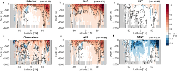
Figure 1. Multi-model zonal mean (global) ocean temperature change, shown as the difference between 2012–2006 mean and 1955–1980 mean for simulations with different forcings, as labelled: (a) historical ALL-forcing; (b) greenhouse gas-only forcing; (c) natural-only forcing; (d) observed changes (Levitus et al 2012); (e) anthropogenic forcing; (f) other anthropogenic forcing (e.g. aerosols). The numbers in brackets (denoted as 'corr') for each model simulation panel indicates the pattern correlation with the observations, omitting missing values. (See figures S1–S3 for the zonal mean of individual basins).
Download figure:
Standard image High-resolution imageTo quantify the individual contributions from different forcings which explain the observed changes in the ocean heat content, we carried out an ROF detection and attribution analysis using multiple combinations of fingerprints (sections 2.1 and 2.2). We make use of volume-averaged temperature, and all model responses were masked according to observational coverage at each depth level and at each time step (section 2.2). Since the dimension of the analysis is limited by the length of pre-industrial control samples needed for the detection and attribution analysis, we make use of global mean time-series calculated for the three representative depth layers instead of zonal mean plots (this is because zonal mean plots would have a much larger spatio-temporal dimension, therefore, requiring a much larger sample of control simulations to provide sufficient estimates of noise from internal variability; Ribes et al 2013).
First, we consider different combinations of inputs for analyses described in table 1. In case B1, (table 1), from an ensemble mean of ALL-forcing simulations and NAT-only simulations, we derive scaling factors  (figure 2(a)), to estimate the respective contribution of the response to anthropogenic and naturally forced responses to observed ocean warming. The anthropogenic signal in ocean warming is confidently detected and attributed (consistent with unity) at the 5%–95% level. The natural signal is not detected, and the confidence interval on
  scaling factors is wide, due to difficulties in distinguishing it from internal variability in the climate system. However, the contribution by natural forcing to observed ocean temperatures is estimated to be small. Next, we regressed observations onto GHG-only and ANT-only time series (case B1; figure 2(b)), to estimate contributions from greenhouse gases alone (GHG) and other anthropogenic forcings (OANT), such as aerosols and ozone, assuming linear additivity of the forcings (figure S7) and neglecting the small natural response.

Figure 2. Detection and attribution results (scaling factors) for a two-signal analysis: (a) cases A1, A2 (as in table 1), (b) cases B1–B4, and the corresponding reconstructed time series of global mean responses (c), (d) using scaling factors from case A1 (c), and using scaling factors from case B3 (d). The time series in (c), (d) are based on CMIP5 multi-model 5 year non-overlapping means, scaled using the attribution results (a), (b). Shaded areas show the uncertainty in the magnitude of the response (spread of scaling factors) for different depth intervals, as labelled. Left panel shows a two-signal analysis resulting in ANT and NAT contributions, the right panel shows results from a two-signal analysis estimating results from a two-signal analysis resulting in GHG and OANT contributions (case B3). The scaling factors are based on analysis of the time-series for 0–300 m, 300–700 m, and 700–2000, regressed simultaneously and masked according to the observational coverage. Note different vertical scales on the two bottom panels. (See table 1 and section 2.2 for how the time-series were constructed and scaling factors derived. See supplementary material for sensitivity analysis and supplementary table S2 for the values plotted in (a), (b).)
Download figure:
Standard image High-resolution imageTo evaluate the sensitivity of results to explicit consideration of natural forcing, we separated the natural influence from the anthropogenic forcings (case B3), and performed a similar regression (ANT and GHG-only), but with the NAT-only ensemble mean signal removed from the observational time series (figures 2(b) and (d); case B4). Such treatment removes the volcanic signal from observations, to make sure that the scaling factors are not affected by volcanoes. This resulted in similar scaling factors as in the previous case where the natural signal was not removed prior to analysis (figures 2(b); S4), suggesting that not accounting for natural forcings does not bias our detection and attribution results. Given that the amplitude of natural signals is estimated to be likely between a scaling factor of 0 and 1 (figure 2(a)), the similarity of these two cases suggests that there is little influence of natural forcing on long trends; further supported by results estimating  and
and  (figure 2(a)). The uncertainties on
  and
and  are relatively large compared to
  (figure 2), however,
  is still constrained and of similar magnitude to
  (figure 2(b)). This provides us with more confidence in using these results for constraining future projections (section 3.2), as results support the model-simulated response to each forcing separating (with scaling factors close to unity).
Sensitivity analysis with inflating the variance from pre-industrial control runs by a factor of 2, accounts for the possibility that internal variability in the models may be lower than in the real world, resulted in a widening of the 5%–95% range uncertainty range in the scaling factors (figure 2, cases A2, B2, B4), but does not affect our main conclusions.
We also carried out a sensitivity analysis to the time-period chosen, by making the start years differ from the year 1955–1980, in five-year intervals. The scaling factors show some sensitivity to the start year of the time-series (figure S4). For starting years of 1975 or later, the scaling factors have much wider uncertainty ranges, because the period 1975 (or later) to 2012 is shorter, and hence, it is more difficult to seperate the signal from climate variability, even though the anthropogenic signal is stronger then. Estimates of scaling factors are expected to depend on the considered period because the longer the period the better the signal to noise ratio (Hegerl et al 1996, Ribes et al 2017). Since start years between 1955 and 1980 makes little difference to the calculated scaling factors, we focus our main analysis on the scaling factors calculated for the longest period available of 1955–2012.
3.2. Anthropogenic contributions to future thermosteric sea level
Thermosteric sea level rise increases in proportion to the increase in the ocean heat uptake (Kuhlbrodt and Gregory 2012, Trenberth et al 2016). In the top 0–700 m of ocean depths sea level rise is estimated to be 1 mm/year in response to 0.31–0.47 W m−2 ocean heat uptake, and 1 mm/year in response to 0.68 W m−2 heat uptake below 700 m depth, because thermosteric expansion differs with depth (Trenberth et al 2009, Trenberth et al 2016). However, the scaling factors for volume-averaged temperatures are not substantially different when derived from a two-depth analysis (0–300 m and 300–700 m, concatenated), or a three-depth analysis that also includes the bottom ocean 700–2000 m. Therefore, we use the three-depth analysis (as in figure 2, but calculated only for models that had sea level rise data), to estimate future thermosteric sea level rise projections due to anthropogenic forcing.
Using such a scaling approach to constrain the future projections is based on the assumption that if a model overestimates a magnitude of historical climate change, the future climate change will be overestimated in a proportional amount (Stott and Kettleborough 2002, Mueller et al 2016, Shiogama et al 2016, Li et al 2017). This approach can be applied to both global mean changes as well as spatio-temporal changes (Shiogama et al 2016) under scenarios where radiative forcing is increasing over time, and the relative contribution of the anthropogenic forcing remains constant over time, which is not the case in all RCP scenarios (Li et al 2017). We applied this approach to the Representative Concentration Pathway (RCP) 8.5 scenario (Vuuren et al 2011), which entails high levels of greenhouse-gas radiative forcings that continually increase over time, and RCP 4.5 scenario, where greenhouse-gas radiative forcings increase at a lower rate and start to stabilize before the year 2100 (figure S7). The present-day aerosol forcing is stronger than future aerosol forcing projections (as in RCP 8.5 or RCP 4.5 scenarios), but the greenhouse-gas forcing is the dominant component of anthropogenic forcing in the future RCP 4.5 and RCP 8.5 scenarios. Since the individual-forcing simulations are not available beyond the year 2012, we use  to scale future projections (as in Li et al 2017), which are dominated by the greenhouse gas forcing. The assumption that the true underlying scaling factors are assumed to be constant is part of the key assumptions behind regression models. Therefore our treatment applied in section 3.1 (using
  for the longest period considered) is consistent with standard detection and attribution assumptions that a model can under or overestimate the magnitude of the response to GHG, but is (assumed) correct in simulating the response pattern over time and with depth, which is to a large part governed by climate physics.
Specifically, to estimate contributions to the future thermosteric sea level rise due to greenhouse gases (figure 3(b)), we make use of the  scaling factors derived as above for the two-signal analysis (figure 2(b); case B3 and B4). Making use of
  scaling factor avoids confounding effects from aerosols (which are also part of the anthropogenic (ANT) forcing). Aerosol emissions decline and get close to zero in RCP 4.5 and 8.5 scenarios (resulting in an increase radiative forcing; figure S7). This scaling factor (
 cases B3 and B4) had the natural signal subtracted from observations in order to remove influences of volcanic activity (see the next section 3.3). Such treatment avoids the situation where the omitted natural forcing signal confounds the estimated signal magnitudes and with its scaling factors. For comparison, we also show the thermosteric sea level results scaled by
  (figure 3(c)), which did not have the natural (volcanic) influence removed. Note that in the near term, decreases in aerosol forcing may lead to a further regional sea level trend (see discussion in conclusion section). However, there are not sufficient future aerosol-only simulations available to fully explore this.
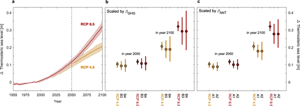
Figure 3. (a) Time series of global mean thermosteric sea level rise changes based on RCP 8.5 (red), and RCP 4.5 (orange) scenarios. Shaded areas show the spread of the four CMIP5 models considered that had sea level data available (table S1), de-trended based on the respective pre-industrial control runs; (b) The vertical bars show the uncertainty spread in the year 2050, and the year 2100, as labelled, with the diamonds and circles indicating the mean value. Lines with circles show thermosteric sea level contributions due to greenhouse gas forcing and anthropogenic forcing (based on the CMIP5 mean in (a)), scaled by  factors (5%–95% CI and mean value) derived from a two-signal analysis, for cases B3 and B4, as labelled; (c) same as (b) but scaled by
  instead. In each group in (b), (c), the first line with a diamond indicates the CMIP5 original model spread (with no scaling), as in (a). Note: The scaling factors were derived for the set of four models used in this plot (table S1) and are similar to those shown in figure 2(b). Anomalies are calculated with respect to the 1955–2012 period (to be consistent with the way the scaling factors were derived). Therefore, these results are not directly comparable with IPCC AR5 SPM.9 figure, due to different base periods and a possibly different set of models used. Sea level rise time-series were de-trended by removing linear trends fitted to pre-industrial control simulations.
Download figure:
Standard image High-resolution imageSince fewer models had global mean thermosteric sea level rise available, we calculated  for the set of models (table S1) that is used for thermosteric sea level projections in RCP 8.5 and RCP 4.5 scenarios. The scaling factors derived in a two-signal analysis show little sensitivity to the set of models chosen (figure S5). Such analysis provides estimates of the increase in thermosteric sea level rise due to greenhouse-gas forcing (figure 3).
An earlier study by Slangen et al (2014) derived the anthropogenic scaling factor  of 1.08 ± 0.13 (±2 σ) by inferring sea level rise from interpolated (full coverage) observations of the ocean heat content prior to detection and attribution analysis performed directly on the sea level time-series. This is broadly consistent with our
  estimates 0.86 (5%–95% range of [0.69, 1.05]; figure S5; supplementary table S2) and similar to our values of
  of 0.91 (5%–95% range of [0.67, 1.17]), since GHG forcing is the dominant component of the anthropogenic forcing (ANT). In contrary to the Slangen et al (2014) study, we obtained the scaling factors by first regressing the raw (non-infilled) observations of the ocean warming on the volume-averaged temperature in CMIP5 models masked by the observational coverage. We then apply these scaling factors to the past and future thermosteric sea level rise (figure 3).
An estimate of thermosteric sea level rise due to greenhouse gas contributions (i.e. thermosteric sea level rise scaled by  ) results in a lower upper bound on sea level rise in both RCP scenarios and a lower mean (by approximately 15%), but a wider uncertainty spread between lower and upper bounds of (5%–95% CI; figures 3; S5). The wider range of the future sea level spread scaled by
  and
and  is due to the fact that we use the mean value (and the 5%–95% lower and upper bounds, figures 3; S5) to scale the ensemble mean sea level rise to all forcings (as in RCP 8.5 or RCP 4.5, respectively). Our results suggest that estimated anthropogenic contributions to future sea level rise projections support the multi-model mean projection range, with stronger support for the central and lower part of the distribution. These findings are consistent with earlier studies which suggested that sea level rise projections from CMIP5 models are consistent with observations albeit may be biased high (Church et al 2013, Nerem et al 2018).
3.3. The role of volcanic activity
Applying the scaling factors obtained from the historical period to scale future thermosteric sea level rise projections is subject to assumptions that solar and volcanic activity has not shown a strong influence on long-term sea level rise over the analysis period. To evaluate the sensitivity of our results to natural forcing (that is dominated by volcanic activity), we have removed the model-simulated natural influence from observations, and performed a similar regression as cases B1 and B2 (ANT and GHG-only; figures 2(b) and (d); cases B3 and B4). Since results were found to be not sensitive to this removal of the solar and volcanic signal from observations, this suggests that scaling factors are not much affected by natural forcing, at least, if the model simulated time-depth response to it. This response is further evaluated in this section.
Natural forcing in the models, and probably also in observations (Schurer et al 2013), is dominated by the response to volcanic eruptions. In order to evaluate the model simulated time-depth pattern of the volcanic response, we analysed the response of ocean warming to volcanic eruptions in an epoch analysis (figure 4) , similar to Iles and Hegerl (2014). It is based on the ocean temperature response to three main volcanic eruptions (Agung, El Chichon, and Pinatubo), occurring in years 1963, 1982, and 1991, respectively. Averaging across the model response in ocean warming to volcanic eruptions reduces internal variability (Iles and Hegerl 2014), and allows for investigation of how deep the volcanic signal penetrates the ocean depths, and how long it extends. In the epoch analysis, time series of the ocean response are identified from 8 years prior to each eruption, to 14 years after the eruption, and averaged across all three eruptions, centered on the eruption year as year '0' (figure 4). Observations were de-trended by removing a linear trend fitted to the whole period (1955–2012), to remove an estimate of the anthropogenic trend. Similarly, for each model, ALL-forcing simulations were masked according to the observational coverage and de-trended in the same way as the observations. Then, an epoch analysis from the three eruptions was conducted. A multi-model mean and range of each individual model simulation's analysis was then taken. The model response is generally consistent with the observed response to natural forcing (estimated by the de-trended observations) (figure 4). The main influence of volcanic activity is noticeable in the top 0–300 m of the ocean depth layer, with the model mean response occurring slightly earlier and recovering later than the observations (figure 4). The response decays within about a decade (note that the temperature drop towards the end may be due to the eruption of Mount Pinatubo within the analysis period for Agung). Results show that model-simulated and observed responses appear broadly consistent, supporting the removal of the model simulated natural forcing response. Our volcanic analysis further shows that if a volcanic eruptions was to occur in the future, the observed time-depth response would probably be reasonably simulated by the models, and could be superimposed on the anthropogenic forced trend.

Figure 4. Epoch analysis for the ocean response to three volcanic eruptions. The response is calculated from de-trended observations (black) and model responses (de-trended, to remove anthropogenic contribution, processed in the same way as the observations), for different depth levels, as indicated. Shaded areas show 5%–95% ensemble envelope average of the epoch analysis.
Download figure:
Standard image High-resolution image
3.4. Uncertainties and limitations
The CMIP5 models used in this analysis do not include ice sheets, therefore actual sea level rise would be higher than the thermosteric sea level rise presented here. Thermal expansion contributes to 30%–50% of the total sea level rise projections (Church et al 2013). Also, our estimates of the anthropogenic and greenhouse-gas attributable components of future thermosteric sea level rise are subject to the assumption that the scaling factors derived from the historical and present-day period can be applied to the future projections (see discussion in section 3.2).
Using multi-model ensemble means, instead of individual model results in detection and attribution framework was shown to generate over-confident scaling factors (Schurer et al 2018). However, due to limited ensemble sizes for the models that had data available (table S1), we resort to using multi-model means to ensure the sample sizes are suitable for the ROF method chosen here. Our sensitivity analysis (figure S4) with inflated variance may at least partly account for that, and shows larger uncertainty rages (5%–95%) on the scaling factors.
We use only one observational dataset Levitus et al (2012), as results from other detection and attribution studies shown to be relatively insensitive to the use of other observational data sets (Gleckler et al 2012, Bilbao et al 2019, Slangen et al 2014). The Levitus et al (2012) dataset provides a raw (non-interpolated) three-dimensional ocean temperature data set, which is needed for detection and attribution analysis presented here (figure S6). Alternative datasets (e.g. Cheng et al 2017) are available, however, in their mapping method (to infill missing data regions in 0–700 m layer), they make use of spatial covariance of CMIP model outputs (Cheng et al 2017). Such products are generally avoided in detection and attribution analyses, because if the observed product was already informed by CMIP model output, then scaling factors that show the amplitude of model fingerprint in observations would no longer be driven by observations only, making the analysis slightly circular (e.g. Hegerl and Zwiers 2011).
4. Conclusions
Previous detection and attribution studies primarily focused on separating natural signal and the forced responses due to all anthropogenic forcings. Here, we advance on previous work by attributing changes in the ocean warming to greenhouse gases alone. The  estimates 0.86 (5%–95% range of [0.69, 1.05]) is similar to the values of
  of 0.91 (5%–95% range of [0.67, 1.17]), since GHG forcing is the dominant component of the anthropogenic forcing (ANT). We find that volcanic cooling was found to be consistent with observations, primarily affecting the top 0–300 m of the ocean. We also use multiple ways of estimating the anthropogenic and greenhouse gas-only signals, to derive scaling factors, which we then use to estimate anthropogenic contributions to the future thermosteric sea level projections. Our results suggest that the mean thermosteric sea level rise in CMIP5 models in response to RCP 8.5 and RCP 4.5 scenarios may be biased high. The estimated greenhouse-gas contribution of the future thermosteric sea level rise supports the multi-model mean projection range, with stronger support for the central and lower part of the distribution. Since the aerosol forcing declines in both RCP 8.5 and RCP 4.5 scenarios, it seems more relevant to scale the future projections by
  which does not include aerosol forcing. However, if, in reality,
  is at the upper end of the range that is consistent with the observations, this could lead to faster sea level rise than in our estimates. Especially in case of future reductions of aerosol emissions (which we neglect for the future in this scaling approach), could lead to a more positive forcing and thus, a more rapid sea level rise in the near-term.
Acknowledgments
We are grateful for helpful comments from Jonathan Gregory, Francis Zwiers, Sybren Drijfhout, Jennifer Mecking, and Andrew R Friedman. We also thank Tim Boyer for assistance with understanding the observational data.
KBT and GCH were supported by the UK NERC-funded SMURPHs project (NE/N006143/1). GCH was further funded by the Wolfson Foundation and the Royal Society as a Royal Society Wolfson Research Merit Award (WM130060) holder. G C H and A P S were supported by the ERC funded project TITAN (EC-320691), and the UK NERC under the Belmont forum, Grant PacMedy (NE/P006752/1).
We acknowledge the World Climate Research Programme's Working Group on Coupled Modelling, which is responsible for CMIP, and we thank the climate modelling groups for producing and making available their model output. For CMIP the US Department of Energy's Program for Climate Model Diagnosis and Intercomparison provides coordinating support and led development of software infrastructure in partnership with the Global Organization for Earth System Science Portals.
Data availability:
All data used is publicly available from the following sources:
CMIP5 data can be accessed at: https://cmip.llnl.gov/cmip5/availability.html
Ocean warming data/volume-averaged temperature, is available at: https://nodc.noaa.gov/OC5/3M_HEAT_CONTENT/
The ROF detection and attribution package developed by Aurélien Ribes is available at https://umr-cnrm.fr/spip.php?article23&lang=fr
Competing interests:
The authors declare no competing interests.