


Abstract
Mexico's government enacted an energy reform in 2013 that aims to foster competitiveness and private investment throughout the energy sector value chain. As part of this reform, it is expected that extraction of oil and gas via hydraulic fracturing will increase in five shale basins (e.g. Burgos, Sabinas, Tampico, Tuxpan, and Veracruz). Because hydraulic fracturing is a water-intensive activity, it is relevant to assess the potential water availability for this activity in Mexico. This research aims to quantify the water availability for hydraulic fracturing in Mexico and identify its spatial distribution along the five shale basins. The methodology consisted of a multilayer geospatial analysis that overlays the water availability in the watersheds and aquifers with the different types of shale resources areas (e.g. oil and associated gas, wet gas and condensate, and dry gas) in the five shale basins. The aquifers and watersheds in Mexico are classified in four zones depending on average annual water availability. Three scenarios were examined based on different impact level on watersheds and aquifers from hydraulic fracturing. For the most conservative scenario analyzed, the results showed that the water available could be used to extract between 8.15 and 70.42 Quadrillion British thermal units (Quads) of energy in the typical 20–30 year lifetime of the hydraulic fracturing wells that could be supplied with the annual water availability overlaying the shale areas, with an average across estimates of around 18.05 Quads. However, geographic variation in water availability could represent a challenge for extracting the shale reserves. Most of the water available is located closer to the Gulf of Mexico, but the areas with the larger recoverable shale reserves coincide with less water availability in Northern Mexico. New water management techniques (such as recycling and re-use), more efficient fracturing methods, shifts in usage patterns, or other water sources need to be identified to allocate water for hydraulic fracturing without affecting current users (e.g. municipal, irrigation, industrial, and environmental flows).
Export citation and abstract BibTeX RIS

Original content from this work may be used under the terms of the Creative Commons Attribution 3.0 licence.
Any further distribution of this work must maintain attribution to the author(s) and the title of the work, journal citation and DOI.
1. Introduction
1.1. Background
In 2013, Mexico passed eleven national structural reforms to modernize the country's economy. One of the most relevant is the energy reform approved in December 2013 [1]. Before the energy reform, Mexico's government monopolized the oil and gas industry for approximately 70 years, and the electricity sector for around 55 years. This reform ends this monopoly with the intent of boosting Mexico's energy industry by fostering competitiveness and private investment throughout the energy value chain [2]. In particular, in oil and gas projects, private investment is expected through service contracts, profit sharing agreements, and licenses [3]. Mexico's Oil Company (Pemex) will transform into a company of the state that will collaborate through profit and/or production sharing agreements [4].
Separately, the use of horizontal drilling and hydraulic fracturing (HF) in the United States enabled extraction from gas and tight oil shale reserves previously deemed uneconomic, and led to an increase in oil and gas production [5–7]. It is expected that the technologies could enable extraction of Mexico's shale resources, as well. Mexico is considered to be one of the top 10 countries in terms of technically recoverable shale resources in the world [8, 9], and its government expects to triple its current gas production by developing HF wells in its shale basins [10, 11]. Mexico's shale resources are located in 5 main basins which have combined risked technically recoverable reserves (RR) of 545 Trillion cubic feet (Tcf) of gas and 13.1 Billion barrels (Bbbl) of oil [12, 13], equivalent to approximately 636 Quadrillion British thermal units of energy (Quads) [14]. The 5 shale basins in Mexico, described in table 1 and shown in figure 1, are Burgos, Sabinas, Tampico, Tuxpan, and Veracruz. The Burgos and Sabinas basins have the largest RR in Mexico (69.3% and 20%, respectively). Furthermore, around 88% of the RR in the 5 basins are located in the shale gas areas.
Table 1. The largest recoverable reserves (RR) in Mexico are located in the Burgos and Sabinas Basin (around 90%). Furthermore, most of the RR are located in shale gas areas. [12, 13].
| Basin | Area (mi2) | RR Oil (Bbbl) | RR Gas (Tcf) | Energy from RR (Quads) | Percentage of Mexico's RR (%) |
|---|---|---|---|---|---|
| Burgos | 24 200 | 6.3 | 393.1 | 441 | 69.3% |
| Sabinas | 35 700 | 0 | 123.8 | 127 | 20% |
| Tampico | 26 900 | 5.5 | 23.2 | 56 | 8.8% |
| Tuxpan | 2810 | 1 | 1.5 | 7 | 1.1% |
| Veracruz | 9030 | 0.3 | 3.4 | 5 | 0.8% |
| MEXICO | 98 640 | 13.1 | 545 | 636 |
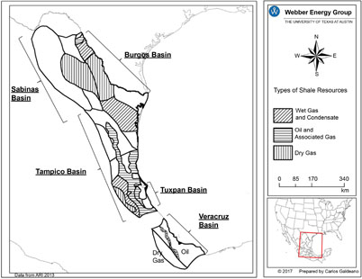
Figure 1 There are 5 continental shale basins in Mexico that have around 636 Quads of recoverable reserves (RR) combined. [12]
Download figure:
Standard image High-resolution imageThe use of HF carries environmental challenges due to (1) the water quantity it requires, and (2) the large volume of wastewater it produces [15, 16]. Impacts vary depending on the water availability and competing demands at a local level [17], but it is important to understand the sources and intensity of water used for HF to evaluate its full impacts on the water resources [18]. Water intensity for HF varies on several factors such as depth, type of shale resources, and thickness of each formation. In shale basins in the United States, HF has required between 1 × 10⁹ and 28 × 109 gallons of water per Quads (gal/Quads) in gas areas, and between 1.5 × 10⁹ and 21.7 × 10⁹ gal/Quads in tight oil areas [19]. In the Eagle Ford Shale formation in Texas, which extends to Mexico, the average water consumption in the oil and gas shale areas, based on the wells estimated ultimate recovery, is 2.6 × 10⁹ and 1.5 × 10⁹ gal/Quads [20]. The estimated ultimate recovery (EUR) is defined as the approximate quantity of shale resource that could be recovered throughout a typical 20–30 year lifetime of a hydraulic fracturing well [20].
Due to the high water demand that HF could cause at a local level [21], different strategies should be analyzed to increase water availability and decrease water stress in the regions where shale resources are located. These strategies could include (1) shifting to less water intensive power plant technologies, (2) shifting to more efficient irrigation technologies, (3) using brackish groundwater as a source of water for HF, and/or (4) recycling and reusing wastewater (e.g. flowback and produced water) that will return to the surface over the lifetime of the HF wells, which in Texas shale areas ranges from 15% to 200% relative to the water demand of the HF wells [22, 23]. For instance, despite the potential increase of water consumption from HF in Texas, it has been shown that in switching from coal-fired to natural gas combined cycle, power plants could reduce water consumption by approximately 60% because of more efficient energy conversion and less water-intensive cooling systems at the power plant [24]. Also, it has been shown that it is possible to increase water availability in the shale regions by using the energy wasted in flared gas activities from HF to treat the flowback and produced water [15]. In 2012, these flared gas in Texas could have been used to treat between 180 and 540 million cubic meters of these wastewater, which is around 1% to 2.4% of Texas' annual water demand [23].
Mexico's water availability varies across the country. Mexico's Water Commission (Conagua) classifies the water availability of the aquifers and watersheds based on four zones that depend on a groundwater availability index (GWAI) and a surface water availability index (SWAI), respectively [26]. These indices are used as thresholds to assign a water price to users [25]. For both indices, the areas classified as Zone 1 represent the areas with greater water scarcity and higher water prices, while the areas classified as Zone 4 have plenty of water available and the water prices range from 10% to 15% of those in Zone 1 areas, depending on the use (e.g. municipal, industrial, agricultural) [25]. Figure 2 shows the classification of Mexico's aquifers and watersheds based on the indices stablished by Conagua. In the northern part of Mexico, most watersheds are classified as Zone 1, while closer to the Gulf of Mexico watersheds are classified as Zone 4. On the other hand, most of the aquifers overlaying the shale areas are classified in a better category (Zones 3 and 4). The aquifers with saline or brackish groundwater are reported every year by Conagua, but the breakdown of the volumes are not reported [27]. Of the aquifers overlaying the shale basins, the Bajo Rio Bravo (No. 1 in figure 2), Cuatrocienegas-Ocampo (No. 2 in figure 2), Paredon (No. 3 in figure 2), and El Hundido (No. 4 in figure 2) have brackish groundwater [27].
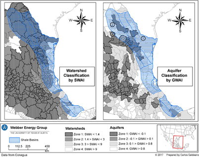
Figure 2 Conagua classifies the water availability of Mexico's watersheds and aquifers in four zones that depend on a GWAI and SWAI. The zones with worst availability overlap with rich oil and gas areas, raising the specter that water scarcity could hinder oil and gas production.
Download figure:
Standard image High-resolution image1.2. Study scope
Even though HF is considered a water-intensive activity, when compared with other high-water users, such as irrigation, it has been relatively small in Texas [21, 28]. Nevertheless, HF has been the major water-intensive user in some counties in Texas [17]. Thus, it is relevant to analyze the potential impacts that it could have on the water resources in Mexico and to quantify the water availability and source (e.g. surface or groundwater) in the different areas where HF wells will be employed.
The main contribution of this study is to develop a methodology to identify the spatial location and volume of water available in the aquifers and watersheds that overlay the five shale basins in Mexico. Furthermore, this letter describes data, methods, and results used to identify the potential EUR energy that could be extracted over the 20–30 year lifetime of HF wells supplied with available surface and groundwater. This research intends to serve as a starting point analysis for the development of strategies for managing new HF demands in the context of constrained water resources.
2. Methodology
The average water availability (WA) for HF in Mexico is estimated by using a multilayer geospatial analysis. This WA considers the average annual surface water and groundwater available to estimate the potential EUR shale reserves that could be extracted from the HF wells that could be supplied with this WA. The surface and groundwater data was provided by Conagua's Water Geographic Information System [29]. These data are based on average values from at least 20 consecutive years of historical records, or from values estimated by Conagua based on other hydrologic parameters (e.g. precipitation, type of soil, evapotranspiration) [30]. The average values are useful as a first approach to determine the WA in the areas analyzed, but future work should incorporate the raw historical data to understand the WA variation during dry and wet periods. Furthermore, the RR in each basin was taken into account in the analysis. The RR in each shale basin was obtained from the report prepared by the Advanced Resources International for the US Energy Information Administration [12]. The potential WA for HF was estimated by intersecting the surface and groundwater availability in each shale area. The methodology is shown in figure 3 and described below.
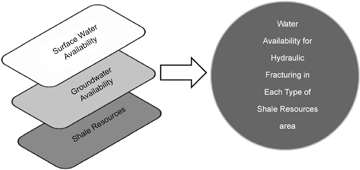
Figure 3 A multilayer geospatial analysis was conducted to determine the water availability in each type of shale resources area in Mexico.
Download figure:
Standard image High-resolution image2.1. Surface water availability
Following Conagua's methodology [31], the mean annual water available in the watersheds (MASWAi) that overlay the shale areas is estimated using equation 1:

where Inputsi and Outputsi are the inputs and outputs of water to the watershed i, as shown in table 2.
Table 2. Four water inputs and five water outputs were considered in each watershed to estimate its water availability.
| Input or Output | Variable | Definition [30] |
|---|---|---|
| Input | Mean annual volume of natural runoff | Natural runoff of the watershed, estimated with either at least 20 years of historical data or the rational method |
| Input | Mean annual volume of runoff from upstream watershed | Water that enters the watershed from the natural drainage of the immediate upstream watersheds. |
| Input | Annual volume of water imports | Water received by the watershed that does not drain naturally from other watersheds or aquifers. |
| Input | Annual volume of water returns | User return flow to the watershed, estimated by either direct measurement or an assumption that depends on type of user. |
| Output | Annual volume of surface water extraction | Water allocated for environmental flows and users registered in the Public Register of Water Rights. |
| Output | Annual volume of water exports | Water allocated to other watersheds in which there is no natural drainage. |
| Output | Annual volume of evaporation in reservoirs | Water evaporated from the reservoirs, estimated based on evaporation measurements applied to the free surface of the reservoir. |
| Output | Annual volume committed to downstream watershed | Water volume needed to drain to the immediate downstream watershed to meet its water users rights and environmental flows |
| Output | Annual volume of variation on storage in reservoirs | Changes in water volume in the reservoirs due to changes in runoff regime, and policies in reservoir operations |
The MASWAiis assumed to be evenly distributed along each watershed i. A ratio is estimated to determine the mean annual surface water available (SWAi) in the intersection of the watersheds and the shale areas using equation 2:
where Ai is the area of the watershed i, and SAkBj∩Ai is the area of the intersection of the watershed i and the shale area k in the shale basin j.
Three different alternatives based on the four zones of WA that Conagua uses to classify Mexico's watersheds are analyzed using the SWAi [26, 27]. The SWAIi for each watershed is estimated using equation 3:

The ranges of the SWAI used to classify Mexico's watersheds by zones are shown in table 3. These zones are based on the WA in each watershed on ascending order from Zone 1 to Zone 4, and are used to determine the water prices. As shown in table 3, the price per cubic meter of water in the watersheds classified as Zone 1, Zone 2, and Zone 3 are 766%, 299%, and 31% more expensive that in Zone 4.
Table 3. Zones of surface water availability and ranges of SWAI, where the best zone is 4 and the worst is 1. Low numbers of the SWAI indicate more water scarcity, which translates into more expensive water for current and new users.
| Zone | Range of SWAI | Increase in water price with respect to Zone 4 |
|---|---|---|
| Zone 1 | SWAI < 1.4 | 766% |
| Zone 2 | 1.4 > SWAI < 3 | 299% |
| Zone 3 | 3 > SWAI < 9 | 31% |
| Zone 4 | SWAI > 9 | — |
The three different alternatives analyzed were:
- Alternative 1. This alternative evaluates the case in which all the SWAi is supplied for HF in the intersection of the watersheds and the shale areas. Under this alternative, new water users could not be added, nor could current users could increase their demand. Also, the water price for all users would be more expensive. This alternative provides an upper bound.
- Alternative 2. This alternative evaluates the case in which part of the SWAi is supplied for HF, but leaving a SWAI>3 (Zone 3). Under this alternative, new users could still be added or current users could increase their water demand, and the water price for all users would either remain the same or increase by around 31%.
- Alternative 3. This alternative evaluates the case in which part of the SWAi is supplied for HF, but leaving a SWAI>9 (Zone 4). Under this alternative, new users could still be added or current users could increase their water demand, and the water price for all users would remain in the cheapest price.
Equation 4 was used to determine the volume supplied for HF in alternatives 2 and 3:
where xi is the water available to be supplied in watershed i by leaving a SWAI greater or equal to 3 or 9 for alternatives 2 and 3, respectively.
2.2. Groundwater availability
Following Conagua's methodology [31], the mean annual groundwater available from the aquifers (MAGWA) that overlay the shale areas were estimated using equation 5:

where Ri is mean annual recharge in aquifer i, NCDi is the natural committed discharge of aquifer i, and GWEi is the extraction of groundwater for other uses. The NCDi is defined as the volume of water from the aquifer committed to springs and rivers, while the GWEi is determined by the volume of groundwater assigned to other users by Conagua [31].
The MAGWAi was assumed to be evenly distributed throughout each aquifer i. A ratio was estimated to determine the mean annual groundwater available (GWAi) in the intersection of the aquifers and the shales areas using equation 6:

where AGi is the area of the aquifer i, and SAkBj∩AGi is the area of the intersection of the aquifer i and the different shale area k in the shale basin j.
In similar fashion as for surface water, three different alternatives were analyzed using the GWAi. These alternatives are based on the four zones of groundwater availability that Conagua uses to classify Mexico's aquifers using a groundwater availability index (GWAI) [25, 32]. The GWAIi for each watershed is estimated using equation 7:

The ranges of the GWAI used to classify the aquifers by zones are shown in table 4. These zones are based on the WA in each aquifer in ascending order from Zone 1 to Zone 4 and are used to determine the water prices. As shown in table 4, the price per cubic meter of water in the aquifers classified as Zone 1, Zone 2, and Zone 3 are 921%, 295%, and 38% more expensive than in Zone 4.
Table 4. Zones of groundwater availability and ranges of GWAI where the best zone is 4 and the worst is 1. Low numbers of the GWAI indicate more water scarcity.
| Zone | Range of GWAI | Increase in water price with respect to Zone 4 |
|---|---|---|
| Zone 1 | GWAI < −0.1 | 921% |
| Zone 2 | −0.1 > GWAI < 0.1 | 295% |
| Zone 3 | 0.1 > GWAI < 0.8 | 38% |
| Zone 4 | GWAI > 0.8 | — |
The three different alternatives analyzed were:
- Alternative 1. This alternative evaluates the case in which all the GWAi is supplied for HF in the intersection of the aquifers and the shale areas. Under this alternative, new water users could not be added, nor could current users could increase their demand. Also, the water price for all users would be more expensive. This alternative provides an upper bound.
- Alternative 2. This alternative evaluates the case in which part of the GWAi is supplied for HF, but leaving a GWAI > 0.1 (Zone 3). Under this alternative, new users could still be added or current users could increase their water demand, and the water price for all users would either remain the same or increase by around 38%.
- Alternative 3. This alternative evaluates the case in which part of the GWAi is supplied for HF, but leaving a GWAI > 0.8 (Zone 4). Under this alternative, new users could still be added or current users could increase their water demand, and the water price for all users would remain in the cheapest price.
Equation 8 was used to determine the volume supplied for HF in the alternatives 2 and 3:

where yi is the water available to be supplied from aquifer i by leaving a GWAI greater or equal to 0.1 or 0.8, respectively. For the aquifers with saline water (brackish or marine intrusion) the fresh and saline water are lumped together in the MAGWA. In these aquifers, the water available for new water intensive users, such as HF, could increase since the demand for saline water is typically smaller than for freshwater. Future research has to be conducted to estimate specific availability of saline water in the aquifers overlaying the shale areas.
2.3. Water availability
Three scenarios of WA, described in table 5, for the shale areas in the shale basins were analyzed by intersecting the surface and groundwater availability alternatives.
Table 5. Three water availability scenarios were analyzed from the intersection of the different ground and surface water availability alternatives.
| Scenario | Watershed final classification | Aquifer final classification | Description |
|---|---|---|---|
| Scenario 1 | Zone 1 | Zone 1 | Estimates the WA after leaving the watersheds and aquifers classified as Zone 1 (Intersection of Alternatives 1). This means that no new user could be added or increase its demand, and the water price for all users would be the most expensive. |
| Scenario 2 | Zone 3 | Zone 3 | Estimates the WA after leaving the watersheds and aquifers classified as Zone 3 (Intersection of Alternatives 2). This means more users could still be added or increase its demand, and the water price for all users would either remain the same or increase 30% to 38%. |
| Scenario 3 | Zone 4 | Zone 4 | Estimates the WA after leaving the watersheds and aquifers classified as Zone 4 (Intersection of Alternatives 3). This means more users could still be added or increase its demand, and the water price for all users would be the cheapest. |
3. Findings
The average annual WA was used to determine the EUR energy that could be extracted over the typical 20–30 year lifetime of the annual HF wells that could be supplied in the shale areas of the 5 shale basins in Mexico. For this first-cut analysis, the RR of the shale areas was treated as if it were evenly distributed. Also, it was assumed that the volume of water needed to extract the EUR of gas or oil would be in the same range as in the shale basins in the US, which is shown in table 6.
Table 6. Range of water demand for HF in the different areas in the shale formations in the United States [19].
| Areas | Low water demand (gal/Quads) | Average water demand (gal/Quads) | High water demand (gal/Quads) |
|---|---|---|---|
| Oil Areas | 1.6 × 10⁹ | 8.2 × 10⁹ | 21.7 × 10⁹ |
| Gas Areas | 1 × 10⁹ | 5 × 10⁹ | 28 × 109 |
3.1. Water availability in the Burgos Basin
Figure 4 shows the EUR energy that could be extracted in the 3 scenarios analyzed in the shale areas of the Burgos Basin. The shaded areas represent the areas where at least 80% of the WA is located in each of the shale areas for each scenario. For instance, in Scenario 1 and 2 the WA is equally distributed in the oil area, whereas in Scenario 3 there is no WA at all in this area. For all the scenarios, the WA for the Oil, Wet Gas 1 (northern) and Dry Gas areas is from groundwater, while around 95% of the WA for the Wet Gas 2 area (southern) is from surface water. In Scenario 3, on average an EUR of around 6 Quads could be extracted in this basin while leaving the classification of the water sources in Zone 4. Most of this energy could be extracted in the wet gas area closer to the Gulf of Mexico (Wet Gas 2), and a fewer from the dry gas and northern wet gas areas.
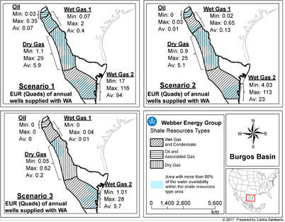
Figure 4 On average, Mexico could extract an EUR of around 100, 28, or 6 Quads over the lifetime of the wells that could be supplied with the average annual WA overlaying the Burgos Basin according to the scenarios analyzed (Scenario 1, 2, and 3 respectively).
Download figure:
Standard image High-resolution image3.2. Water availability in the Sabinas Basin
Figure 5 shows the EUR energy that could be extracted in the 3 scenarios analyzed in the shale area of the Sabinas Basin. The shaded areas represent the areas where at least 80% of the WA is located in the Dry Gas area for each scenario. There is no surface water available in any scenario analyzed. In Scenario 3, on average an EUR of around 0.14 Quads could be extracted in this basin with the WA in the aquifers while leaving its classification as Zone 4.
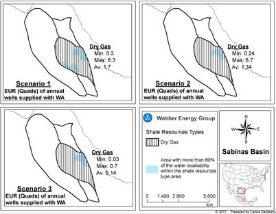
Figure 5 On average, Mexico could extract an EUR of around 1.7, 1.34, or 0.14 Quads over the lifetime of the wells that could be supplied with the average annual WA overlaying the Sabinas Basin according to the scenarios analyzed (Scenario 1, 2, and 3 respectively).
Download figure:
Standard image High-resolution image3.3. Water availability in the Tampico Basin
Figure 6 shows the EUR energy that could be extracted in the 3 scenarios analyzed in the shale areas of the Tampico Basin. The shaded areas represent the areas where at least 80% of the WA is located in each shale area for each scenario. For Scenario 1, most of the WA is from surface water, while in Scenario 2 and 3 the main sources of water varies for each shale area (table 7).
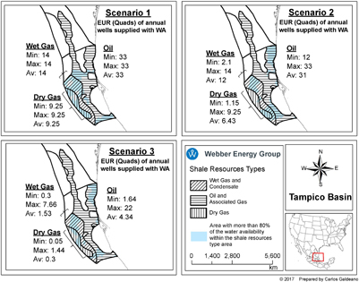
Figure 6 On average, Mexico could extract an EUR of around 56, 50, or 6 Quads in over lifetime of the wells that could be supplied with the average annual WA overlaying the Tampico Basin according to the scenarios analyzed (Scenario 1, 2, and 3 respectively).
Download figure:
Standard image High-resolution imageTable 7. The main source of water available for hydraulic fracturing in the Tampico Basins varies significantly in each scenario and for each type of shale resources area.
| Shale resources | % of WA from surface water | % of WA from groundwater | ||||
|---|---|---|---|---|---|---|
| type area | Scenario 1 | Scenario 2 | Scenario 3 | Scenario 1 | Scenario 2 | Scenario 3 |
| Oil | 99% | 83% | 89% | 1% | 17% | 11% |
| Wet Gas | 99% | 65% | 71% | 1% | 35% | 29% |
| Dry Gas | 99% | 72% | 35% | 1% | 28% | 65% |
As figure 6 shows, in Scenario 1 the maximum, minimum, and average EUR energy that could be extracted is the same in each shale area, which means that the average water that could be supplied to HF wells in one year could extract all the RR in these areas over the lifetime of these wells. In Scenario 3, on average an EUR of around 6 Quads could be extracted, while leaving the watersheds and aquifers classification as Zone 4. Most of this energy could be extracted in the Oil area closer to the Gulf of Mexico, followed by the Wet Gas and Dry Gas areas.
3.4. Water availability in the Tuxpan Basin
Figure 7 shows the EUR energy that could be extracted in the 3 scenarios analyzed in the different shale areas of the Tuxpan Basin. The shaded areas represent the areas where at least 80% of the WA is located for each scenario. For all the scenarios, more than 90% of the WA is from surface water. In Scenario 1, the maximum, minimum, and average EUR energy that could be extracted in the shale oil area of the Tuxpan Basin is the same, which means that the average water that could be supplied to the HF wells in one year could extract all the RR in these areas over the lifetime of these wells. In Scenario 3, on average an EUR of around 0.77 Quads could be extracted, while leaving its watersheds and aquifers classification as Zone 4.

Figure 7 On average, Mexico could extract an EUR of around 7.2, 5.9, or 0.77 Quads over the lifetime of the wells that could be supplied with the average annual WA overlaying the Tuxpan Basin according to the scenarios analyzed (Scenario 1, 2, and 3 respectively).
Download figure:
Standard image High-resolution image3.5. Water availability in the Veracruz Basin
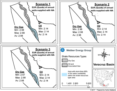
Figure 8 shows the EUR energy that could be extracted in the 3 scenarios analyzed in the shale areas of the Veracruz Basin. The shaded areas represent the areas where at least 90% of the WA is located in each shale area for each scenario. For all the scenarios, more than 95% of the WA in both shale resources type areas (Oil and Dry Gas) is from surface water. In the 3 scenarios, the maximum, minimum, and average EUR energy that could be extracted is the same in each shale area, which means that the average water that could be supplied to the HF wells in one year could extract all the RR in these areas over the lifetime of these wells. The main reason is due to the high WA in the region and the small amount of RR located in these areas. Most of the water is located in the south of the shale areas.
Figure 8 Mexico could extract all the risked technically recoverable resources (around 5 Quads) from the Veracruz Basin over the lifetime of the wells that could be supplied with the average annual WA according to all the scenarios analyzed (Scenario 1, 2, and 3).
Download figure:
Standard image High-resolution image
4. Discussion
For the scenarios analyzed, WA varies along the five shale basins. In some cases there is more WA from surface water than for groundwater, and vice versa. This discussion is based on the results from Scenario 3, which estimates the amount of EUR energy that could be extracted while maintaining the WA indices of the aquifers and watersheds in the best classification possible (Zone 4). The WA estimated in Scenario 3 could be used to extract an EUR between 8.15 and 70.42 Quads, with an average of around 18.05 Quads (table 8). The average EUR energy that could be extracted with the WA represents around 4% of Mexico's RR (around 440 Quads [12]). This average EUR energy would be extracted over the typical 20–30 year lifetime of the HF wells that could be supplied with the WA. This EUR energy would represents around 7% of Mexico's energy consumption in the next 30 years, assuming an annual energy consumption of around 7.5 Quads [33, 34].
Table 8. An EUR between 8.15 and 70.42 Quads, with an average of around 18.05 Quads, could be extracted leaving the watersheds and aquifers in their best corresponding classification (Zone 4).
| EUR energy that could be extracted with the WA in Scenario 3 (Quads) | |||||||
|---|---|---|---|---|---|---|---|
| Shale Basin | Minimum | Average | Maximum | ||||
| From watersheds | From aquifers | From watersheds | From aquifers | From watersheds | From aquifers | ||
| Burgos | 0.99 | 0.06 | 5.54 | 0.32 | 27.70 | 1.62 | |
| Sabinas | 0 | 0.03 | 0 | 0.14 | 0 | 0.71 | |
| Tampico | 1.67 | 0.30 | 5.04 | 1.12 | 25.66 | 5.65 | |
| Tuxpan | 0.28 | 0.01 | 0.75 | 0.02 | 3.83 | 0.13 | |
| Veracruz | 4.80 | 0.01 | 5.11 | 0.01 | 5.11 | 0.01 | |
| TOTAL | 8.15 | 18.05 | 70.42 | ||||
The geographic distribution of the WA varies across the shale areas in each shale basin, which could represent a challenge for extracting the RR. In the Burgos Basin, around 96.5% of the average EUR energy would be from the wet gas area closer to the Gulf of Mexico, representing about 4% of the RR of the combined wet gas areas in this basin (146 Quads [12]). The breakdown from the average EUR energy that could be extracted in this basin from the oil, northern wet gas, and dry gas areas was around 0%, 0.1%, and 3.4%, respectively. This energy represents about 0%, 0.005%, and 0.07%, of RR in the oil (6 Quads [12]), combined wet gas, and dry gas (288 Quads [12]) areas, respectively. The WA for the dry gas and northern wet gas areas would be from groundwater, whereas 98% of the WA for the wet gas area closer to the Gulf of Mexico would be from surface water.
In the Sabinas Basin, there is only groundwater available to extract dry gas in the northeastern area. The average EUR energy that could be extracted from this basin represents about 0.11% of its RR (127 Quads [12]). In the Tampico Basin, around 70%, 25%, and 5% of the total average EUR energy could be extracted from the oil, wet gas, and dry gas areas, respectively. This energy represents about 13%, 11%, and 3%, of the RR in the oil (32 Quads [12]), wet gas (14 Quads [12]), and dry gas (9 Quads [12]) areas, respectively. For the oil and wet gas areas of this basin, around 89% and 71% of the WA is from surface water, whereas for the dry gas area 65% of the WA is from groundwater. For the Tuxpan Basin, around 97% of the WA is from surface water. The average EUR energy that could be extracted from its oil area represents about 11% of its RR (7 Quads [12]). In the Veracruz basin, the EUR energy that could be extracted with the WA is equal to its RR (around 5.12 Quads [12]), which is due to the high surface water availability in the southern region of the shale basin.
5. Conclusion
Water availability varies across each of the five shale basins. Three scenarios were examined based on different impact level on watersheds and aquifers from HF. The most conservative scenario analyzed could assist to determine and identify the potential areas with WA for HF that would not increase water stress and water prices from the watersheds and aquifers overlaying the shale areas. Under this scenario, the average annual water available could be used to supply HF wells that can extract on average 18.05 Quads over a 20–30 year lifetime period, which represents around 7% of the energy that Mexico could consume in 30 years. However, the geographic distribution of the WA could represent a challenge for extracting the shale RR in some areas. Most of this water is located closer to the Gulf of Mexico; whereas the areas with less WA are in Northern Mexico, where the larger reserves are located. Future research has to be conducted to examine (1) a dynamic change in the spatial variables such as water demand growth of municipal and irrigation users, and (2) the water availability variation under extreme conditions (dry and wet years). Furthermore, different strategies should be analyzed to increase WA in the regions where most of the shale resources are located without affecting current users or depleting the water sources. These strategies could include (1) shifting power plant technologies for less water intensive options, (2) shifting to more efficient irrigation technologies, (3) using brackish groundwater as a source of water for HF, and (4) recycling and reusing wastewater (e.g. flowback and produced water) that will return to the surface over the lifetime of the HF wells.
Acknowledgments
The authors would like to thank Mexico's National Council for Science and Technology (Conacyt), The Cynthia & George Mitchell Foundation, and the National Science Foundation CRISP project for funding this research. Also, the authors would like to thank Carlos R Montaño Espinosa of Conagua for providing data from Mexico's aquifers and watersheds. Likewise, the authors would like to thank David T Allen, Elena C McDonald-Buller, Gary R McGaughey, Kimura Yosuke, Sheila M Olmstead, Melinda E Taylor, Felipe J Cardoso-Saldana, Niall Gaffney, Paul Navratil, and Dave Semeraro for their support and insights during the development of this research.