

Abstract
Irrigation is known to influence regional climate but most studies forecast and simulate irrigation with offline (i.e. land only) models. Using south eastern Australia as a test bed, we demonstrate that irrigation demand is fundamentally different between land only and land–atmosphere simulations. While irrigation only has a small impact on maximum temperature, the semi-arid environment experiences near surface moistening in coupled simulations over the irrigated regions, a feedback that is prevented in offline simulations. In land only simulations that neglect the local feedbacks, the simulated irrigation demand is 25% higher and the standard deviation of the mean irrigation rate is 60% smaller. These local-scale irrigation-driven feedbacks are not resolved in coarse-resolution climate models implying that use of these tools will overestimate irrigation demand. Future studies of irrigation demand must therefore account for the local land–atmosphere interactions by using coupled frameworks, at a spatial resolution that captures the key feedbacks.
Export citation and abstract BibTeX RIS

Original content from this work may be used under the terms of the Creative Commons Attribution 3.0 licence.
Any further distribution of this work must maintain attribution to the author(s) and the title of the work, journal citation and DOI.
1. Introduction
One of the primary anthropogenic activities in terms of land use is agriculture that accounts for over USD$3 trillion in global economic activity annually according to the World Bank national accounts data. Future climate change is projected to have large and regionally dependent impacts on future agriculture due to increasing temperatures and altered precipitation (Lobell and Field 2007, Rosenzweig et al 2013). Irrigation expands the area of land suitable for a range of crop types, including wheat and cereals, corn, rice, and fruits and vegetables. The area utilizing irrigation was estimated at around 324 million hectares in 2012, supporting an estimated 40% of the total food production worldwide despite occupying only 20% of the cultivated area (FAO 2016).
Local climate and irrigation are intertwined. Changes in climate affect irrigation rates by increasing evaporative demand. Irrigation affects regional climate primarily through the energy balance by increasing evaporation and decreasing sensible heat exchange, which in combination tend to cool the surface. Simulating irrigation demand and the impacts of climate change on agriculture has traditionally used land only (offline) simulations (Rosenberg et al 2003, Izaurralde et al 2003, De Silva et al 2007, Wisser et al 2008, Liu et al 2013, Mehta et al 2013, Elliott et al 2013, Leng et al 2013, Sun et al 2013, Blanc et al 2014, Wada et al 2014, Anderson et al 2015, Leng et al 2015, Woznicki et al 2015). Offline simulations of future irrigation demand are generally forced using output from coupled climate models. These studies account for how the atmosphere drives irrigation and agriculture but neglect how irrigation impacts the atmosphere. If irrigation occurs over large areas, it can have a significant impact on regional climate. Evaporation is increased by irrigation (Leng et al 2013, Lu et al 2015) which cools and moistens the near surface air (Sacks et al 2008, Huang and Ullrich 2016) reducing the maximum monthly air temperature by up to 7.5 °C in California (Kueppers et al 2007). Because irrigation demand is dynamic, responding to changes in water use, atmospheric conditions, and plant growth, the irrigation induced changes in near surface climate is a feedback on irrigation demand.
The question of how much future climate change affects irrigation demand has direct relevance to future food security. The necessity of including anthropogenic activities such as irrigation has been recently recognized by the international community. The Global Energy and Water Cycle Experiment (GEWEX) is undertaking a joint venture between the GEWEX Global Hydroclimatology Panel (GHP) and the GEWEX Global Land/Atmosphere System Study (GLASS) Panel to include human impacts such as irrigation and water withdrawals in land surface models (LSMs). A major gap in most existing studies is the lack of land–atmosphere feedbacks due to the use of offline simulations to evaluate future irrigation water usage. Given the known impacts of irrigation on regional climate, we examine how seriously projections or hindcasts of irrigation demand will be affected if feedbacks with the local atmosphere are neglected. We use south eastern Australia as a test-case, examining the magnitude of the feedback between irrigation demand and regional climate to ask: Can offline simulations be used to reliably forecast irrigation demand?
2. Methods
2.1. Model systems and approach to irrigation
We assess the impact of irrigation on the local climate and the importance of local feedbacks on simulating irrigation demand using the Land Information System (LIS) version 6. LIS is a National Aeronautics and Space Administration (NASA) developed model framework that facilitates running various land surface models (LSM) coupled to the NASA Unified Weather Research and Forecasting (NU-WRF) atmospheric model. In this study we use NU-WRF coupled to the Community Atmosphere Biosphere Land Exchange (CABLE) LSM (Kowalczyk et al 2006, Wang et al 2011). The configuration and parameterizations for NU-WRF are selected based on previous work (Evans et al 2014, Hirsch et al 2014a, 2014b) and include the Yonsei University scheme, the the Kain–Fritsch cumulus parameterization scheme, the single moment 5-class microphysics scheme, the Rapid Radiative Transfer Model long wave scheme, and the Dudhia short wave scheme. The version of CABLE used in this study includes a groundwater module, and subgrid runoff parameterizations (Decker 2015) in addition to a new pore scale model based formulation for soil evaporation (Decker et al 2017). The phenology in CABLE is prescribed from the observed moderate resolution imaging scanner (MODIS) leaf area index (LAI).
A new crop irrigation module and map of irrigated areas was developed for CABLE to simulate irrigation based on the recommendations from the Australian government for irrigating winter cereal crops. The Australian Government only recommends irrigation at the start of the growing season and when the soil in the entire root zone is dry. Due to the open market for water in the Murray–Darling Basin, it is likely that farmers only irrigate when economically beneficial. Variations of the methodology used here have been used previously to investigate the interactions between irrigation and climate (Kueppers et al 2007, Lu et al 2015). We assume irrigation occurs whenever the following conditions are met:
- 1.It is the winter wheat season and the gridcell is equipped for irrigation.
- 2.The soil moisture in the rooting zone is less than half of the plant available soil moisture in every layer in the root zone (the first 4 of the 6 total soil layers in CABLE).
- 3.It is not raining.
To satisfy condition (1) the winter wheat growing season is specified using typical plant and harvest dates of May 1 and November 1. The planting and harvest dates vary annually due to climate variability as well as with the specific cereal crop planted (Matthews et al 2016). We use a constant growing season length as the relatively short time span of our study precludes large-scale climate driven trends in growing season length. Condition (2) above is satisfied when, for all soil layers, 1 <= i <= 4
Where θi is the volumetric soil moisture content in layer i (mm3 mm−3), θwp is the volumetric soil moisture at wilting point (mm3 mm−3), and θsat volumetric soil moisture at saturation (mm3 mm−3). Condition (3) is checked after conditions (1) and (2) by evaluating the precipitation from NU-WRF. The irrigation amount is calculated as:
where Mirrig is the mass per area (kg m−2) of irrigated water added to the soil column, and Δzi is the layer thickness (mm). The rate of irrigated water is simply:
where Δt is the model timestep. Irrigation is added directly to the existing root zone soil moisture:
Where Δztotal is the total thickness of the root zone (mm), and Mirrig is given by equation (2). To ensure conservation, water used for irrigation is removed from the aquifer module:
where θaq (mm mm−3) is the volumetric water content in the aquifer and Δzaq = 20 000 (mm) is the prescribed thickness of the aquifer layer.
2.2. Data and Experimental Design
The area equipped for irrigation in south eastern Australia is taken from the National Land Use Mapping Project of the National Land and Water Resources Audit of Australia (2013). These data are a compilation of irrigated land boundaries submitted by many agencies and are representative of the important irrigated areas in the region. We used the 3 hourly Princeton dataset (Sheffield et al 2006) to spin-up CABLE prior to the coupled and the land only (offline) simulations, and the ERA-Interim reanalysis (Dee et al 2011) for initial and boundary conditions for the coupled simulations. The coupled simulations are validated using daily maximum near surface air temperature and precipitation from the Australian Water Availability Project (AWAP) (Jones 2009), a gridded, station based product. The evapotranspiration is validated using the MODIS MOD16 evapotranspiration product (Mu et al 2007, Mu et al 2011).
The initial land surface condition for the NU-WRF control (no irrigation) and irrigated experiments were spun-up separately by running CABLE in offline mode within LIS from 1979–2004 Both the control and irrigated simulations consist of six ensemble members. The initial conditions for each ensemble member where varied by starting each a month apart, such that the start dates range from 1 August 2004 to 1 January 2005. Each ensemble member is run from 2005–2010 All simulations are run at a resolution of 10 × 10 km2. The coupled results presented here consist of the ensemble mean of the six ensemble members. In addition to the coupled simulations, an irrigated offline (land-only) simulation is run from 1 January 2005 to 1 January 2011. The irrigated offline simulation is forced with the near-surface output from the ensemble mean of the control NU-WRF simulations. The irrigated offline simulation is initialized with the same land surface state as the irrigated coupled simulation. The differences between the irrigated offline and irrigated coupled simulations from 2005–2010 are due to irrigation-atmosphere feedbacks.
3. Results
3.1. Climate impacts of irrigation
The coupled control simulations accurately reproduce the large temperature and precipitation gradient from the mountains in far southeastern Australia to the much hotter and drier inland regions (figures 1(a)−(d)). Over the irrigated crop lands (figure 1(e)) the differences in mean growing season maximum near-surface air temperature resulting from irrigation is around 0.5 °C (figure 1(f)). Note the precise co-location of the largest (and statistically significant) cooling (indicated with hatching in figure 1(f)) with the irrigation pattern (figure 1(e)). In the regions surrounding the irrigation, the impact on growing season near-surface maximum daily air temperature is slightly negative (0.1–0.2 °C) but not statistically significant. Irrigation also moistens the near-surface air (figure 2). The mean specific humidity in the control simulation is around 5 g kg−1 and including irrigation increases the specific humidity by 0.2–0.5 g kg−1 or around 5%–10%. Similar to the maximum daily temperature, the statistically significant increase in specific humidity is limited to regions of irrigation. Irrigation does not significantly alter the surface radiation budget (downward shortwave and longwave radiation) or precipitation (not shown). It is not surprising that the precipitation remains unchanged; precipitation during the winter wheat season is governed by large-scale synoptic patterns and not localized convective events. The statistically significant impacts of irrigation on the climate in south eastern Australia are therefore limited to cooling and moistening the atmosphere above the irrigated areas. Note, we do not show results from the uncoupled simulations here because by definition there are no changes in near-surface air temperature or specific humidity.
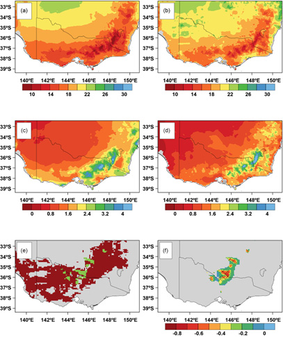
Figure 1 The mean maximum temperature at two meters above the surface during the growing season from (a) observations and from (b) the coupled control simulations, the mean precipitation rate (mm day−1) from the (c) observations and the (d) coupled control simulations. Also shown is (e) the irrigated croplands (blue) and the rain fed croplands (white), and (f) the difference in mean maximum two meter air temperature between the coupled irrigated and coupled control simulations. The hatching in (f) indicates where the differences are significant at the 95% confidence level using a standard t-test.
Download figure:
Standard image High-resolution image3.2. Irrigation demand
The mean rate of irrigation for the offline and coupled simulations is shown in figure 3(a) as a function of the mean near-surface humidity from the first model level in NU-WRF. The offline simulations are forced using the specific humidity from this level but it is a prognostic variable in the coupled simulations. The offline simulations generally have a higher irrigation rate ranging from 1.5–2.4 mm day−1 with an average value of 1.8 mm day−1. In contrast the coupled simulations frequently have lower irrigation rates that range from 0.1–2 mm day−1 with an average of 1.4 mm day−1. The variability in the irrigation rate is larger for the coupled simulations than the offline (figure 3(b)). The offline simulations show irrigation rates predominantly around 1.75 mm day−1 with only 10% of grid cells with a rate less than 1.55 mm day−1, while the coupled simulations have significant number (60%) of grid cells with irrigation rates less than 1.55 mm day−1. The standard deviation of the mean irrigation rate is 0.14 mm day−1 in the offline simulation and 0.35 mm day−1 in the coupled simulations. The mean irrigation rate is therefore 25% larger and the variability in the mean irrigation rate is 60% smaller than the coupled simulations. The total evaporative fluxes (E) over the irrigated croplands are larger in the offline simulation than the coupled simulations (figure 4) throughout the year. As expected, the coupled and offline simulations that include irrigation have a much larger seasonal cycle of E than the simulations without irrigation. The offline simulations with irrigation have an annual maximum in E around 1.75 mm day−1 that lasts from September–November. In contrast the coupled simulations have a strong peak in E of 1.5 mm day−1 that falls quickly to a value similar to the control simulation. The mean E from the offline simulations is 1.1 mm day−1 but only 0.8 mm day−1 for the coupled simulations.
4. Discussion
The physical mechanisms underpinning the differences between the offline and coupled simulations relate primarily to E and the near-surface humidity. In the offline simulations (figure 4) E greatly exceeds the observations and lasts throughout the growing season, depleting the soil moisture thereby requiring more irrigation to be applied. The higher E does not affect near-surface humidity; the nature of offline experiments breaks this feedback relationship, and so the high E does not increase the near-surface humidity and thereby reduce E. In contrast, in the coupled experiments, E decreases more rapidly after peaking, similar to the observations. The reduction in E causes more soil moisture to be retained and therefore less irrigation is applied in the coupled simulations. The E prior to the onset of irrigation is similar for the irrigated and non-irrigated coupled simulations and the observations, while the offline simulations retain a higher value of E throughout the year. The near-surface humidity (figure 3(a)) is slightly larger in the coupled simulations as the boundary layer moistens following irrigation.
The necessity of using coupled land–atmosphere simulations for accurately simulating irrigation demand with a process based model in semi-arid regions stems from the feedback of near-surface humidity on the total evaporative flux from the surface. The humidity in the first model level in NU-WRF is moistened due to the increased evaporative flux due to irrigation (figure 2). However the offline forcing data has no information regarding the previous moisture fluxes, and it remains dry despite the increased moisture fluxes following irrigation. In the coupled runs the increased humidity in the planetary boundary layer (PBL) feedbacks into evaporation, reducing the total moisture flux from the surface. The impact of PBL moistening can be assessed using a simple parameterization for turbulent moisture fluxes from the surface:
where E is expressed in mm s−1, qsrf (kg kg1) is the specific humidity at the surface, qatmo (kg kg1) is the specific humidity in the atmosphere near the surface, r is the resistance to turbulent transfer, and β represents water limitation. Assuming that the increased E induces a increase in the atmospheric specific humidity of Δq and qsrf remains constant, the difference in flux (ΔE) due to local land–atmosphere feedbacks is:

Figure 2 The mean growing season near surface specific humidity (g kg−1) in the coupled simulation without irrigation (a), the difference between the irrigated and non-irrigated coupled simulations (b), and the difference between the irrigated and non-irrigated coupled simulations regridded to a standard climate model grid (c). The statistically significant (at 95%) differences between the control and irrigated simulations are shown with hatching in (b).
Download figure:
Standard image High-resolution imageUsing typical values of r = 100 s m−1, β = 1.0 (representing the wet conditions during irrigation), and taking Δq = 0.0006 kg kg−1 figure 2(b), the reduction in E associated with surface air moistening is −6 × 10⁻⁶ mm s−1, or −0.5 mm day−1. This value is similar to the difference in mean irrigation rates 0.4 mm day−1 (figure 3(a)). The value also agrees reasonably well with the difference E (0.3 mm day−1) between the coupled and offline simulations. Despite neglecting the differences in stability, ground temperature, and the time evolution of the nonlinear system, equation (7) yields the correct order of magnitude for the observed discrepancies between the offline and coupled simulations. Neglecting this feedback using only offline simulations will always lead to computing too much irrigation due to the elevated E flux caused by the failure to allow E to moisten the PBL.
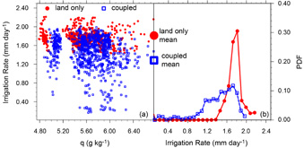
Figure 3 (a) Mean irrigation rate versus near surface specific humidity (q) for each year from 2005–2010 for the. coupled simulations (blue squares) and the offline simulations (red circles). Also shown is the spatially averaged mean irrigation rate on the right hand side of panel (a). (b) The probability density function (PDF) of the mean irrigation rate for the coupled (blue line with squares) and the offline (red line with circles).
Download figure:
Standard image High-resolution image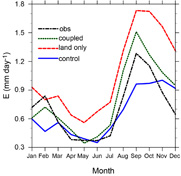
Figure 4 Monthly climatology of the total evaporative flux from the surface (E in mm day−1) averaged over the irrigated areas from the coupled control simulation (labelled control), the coupled simulation including irrigation (labelled coupled), the offline simulation with irrigation (labelled land only), and from observations (labelled obs).
Download figure:
Standard image High-resolution image
The increase in near-surface humidity in figure 2(b)) is largest directly over the irrigated areas, suggesting that it will not be fully captured if the model resolution is coarse compared to the irrigated area. The feedback is resolved in our simulations because the irrigated regions occupy the entire grid cell due to the high spatial resolution (10 × 10 km2). However, if the model resolution is coarse compared to the irrigated area the feedback on the atmosphere will be weaker. The Community Atmosphere Model (CAM) sub-divides each grid cell into multiple tiles and frequently employs a resolution of 1.9° × 2.5°. The irrigation rate in a coarse resolution, tiled simulation is calculated for the irrigated tile using the atmospheric forcing from the entire grid cell. Similar to using land only simulations, in regions where the irrigated fraction of the grid cell is small relative to the total area, the local atmospheric feedback will likely by unresolved and lead erroneous irrigation rates. To approximate how the grid cell mean atmospheric state would change if our study utilized a coarse resolution climate model, figure 2(c) shows the response of the near-surface atmospheric humidity averaged to a resolution representative of climate modeling studies (1.9° × 2.5°). While climate models aggregate the fluxes from each tile to the grid cell mean at each timestep, averaging our results to a coarse resolution provides a first estimate to how a climate model could respond when only a small portion of the grid cell is irrigated. Due to the small areal extent of the irrigation, the area averaged increase in q is an order of magnitude smaller than what occurs directly over the irrigated crops (in figure 2(c) one grid cell has a value of 0.055, others are near 0.02 g kg−1). Using equation (7) it is evident that E will be too large leading to excessive irrigation rates. The actual value of Δq due to irrigation in a coarse resolution climate simulation will differ from our approximation yet will be less than Δq when the entire grid cell is irrigated. The use of a tiled land surface representation when the irrigation area is small relative to the resolution of the model will necessarily lead to a diminished near-surface feedback.
Prior research has not quantified the impact of the near-surface feedback, but they do offer insight into methods to deal with it. Recent work by Huang and Ullrich (2016) using a variable resolution atmospheric model to simulate irrigation demonstrates a possible future research direction. Variable resolution climate models allow small scale features, such as localized feedbacks over irrigated regions, to be captured. Alternatively, Leng and Tang (2014) calibrated the irrigation amounts to observed values using offline simulations. This approach neglects the fundamental reason why the irrigation amounts are incorrect. Studies of future irrigation demand using calibrated irrigation amounts and neglecting this first order feedback cannot properly simulate how irrigation rates will change over time as the climate changes. Future work utilizing physically based simulations of irrigation rates must account for the localized feedbacks even if irrigation is explicitly included in a coarse resolution climate model.
The reported mean irrigation rate in 2014–2015 for pastures and wheat in Southeastern Australia varies with the region between 2.0–3.6 Mg ha−1 or 0.6–1.0 mm day−1 (Australian Bureau of Statistics, 2016), below the mean estimate from the coupled (1.4 mm day−1) and offline simulations (1.8 mm day−1). The coupled simulations exhibit more points (figure 3(a)) in better agreement with the mean reported irritation rates. The descrepency is likely due to the simple irrigation module that does not account for how individual farmers will minimize water usage to minimize cost. Future research into physcially based simulations of irrigation demand in the region will need to account for these factors.
Offline experiments are common in many areas of land surface science and commonly prove useful in diagnosing errors (e.g. Best et al 2015). However, in experiments designed to assess phenomenon, where changes in the phenomenon feed back strongly with the atmosphere, coupled experiments should be conducted wherever possible.
5. Conclusions
Forecasting future irrigation demand under a changing climate requires knowledge of agricultural practices, water availability, economics concerning water usage, and an accurate representation of physical processes. This study demonstrates that local feedbacks between the atmosphere and the land surface are of first order importance for accurately simulating irrigation demand in semi arid regions. Neglecting the moistening of the PBL, the direct result of increases in the surface to atmosphere moisture fluxes from irrigation, increases the total simulated irrigation demand by 25% and decreases the standard deviation in the mean irrigation rate by 60%. Studies that take output from global climate models to drive land-only models neglect this important effect, and will lead to erroneous conclusions about future irrigation water demand. Similarly, coarse resolution climate models that includes irrigation will not adequately resolve the local land–atmosphere feedbacks that limits irrigation demand in semiarid regions when the irrigated area is small compared to the model grid resolution.
Acknowledgments
This work was supported by the ARC Centre of Excellence in Climate Systems Science. The irrigation cover map is available from https://data.gov.au.