

Abstract
Phenology deals with timing of biotic phenomena and seasonality concerns temporal patterns of abiotic variables. Studies of land surface phenology (LSP) and land surface seasonality (LSS) have long been limited to visible to near infrared (VNIR) wavelengths, despite degradation by atmospheric effects and solar illumination constraints. Enhanced land surface parameters derived from passive microwave data enable improved temporal monitoring of agricultural land surface dynamics compared to the vegetation index data available from VNIR data. LSPs and LSSs in grain growing regions of the Volga River Basin of Russia and the spring wheat belts of the USA and Canada were characterized using AMSR-E enhanced land surface parameters for the period from April through October for 2003 through 2010. Growing degree-days (GDDs) were calculated from AMSR-E air temperature retrievals using both ascending and descending passes with a base of 0 ° C and then accumulated (AGDD) with an annual restart each 1 April. Tracking the AMSR-E parameters as a function of AGDD revealed the expected seasonal pattern of thermal limitation in mid-latitude croplands. Vegetation optical depth (VOD), a microwave analog of a vegetation index, was modeled as a function of AGDD with the resulting fitted convex quadratic models yielding both high coefficients of determination (r2 > 0.90) and phenometrics that could characterize cropland differences between the Russian and North American sites. The AMSR-E data were also able to capture the effects of the 2010 heat wave that devastated grain production in European Russia. These results showed the potential of AMSR-E in monitoring and modeling cropland dynamics.
Export citation and abstract BibTeX RIS

Content from this work may be used under the terms of the Creative Commons Attribution 3.0 licence. Any further distribution of this work must maintain attribution to the author(s) and the title of the work, journal citation and DOI.
1. Introduction
Phenology and seasonality are complementary aspects of ecosystem functioning: phenology deals with timing of biotic phenomena; whereas, seasonality concerns temporal patterns of abiotic variables. Land surface phenology (LSP) describes the timing of vegetated land surface dynamics as observed by remote sensing at spatial resolutions and extents relevant to meteorological processes in the atmospheric boundary layer (de Beurs and Henebry 2004, 2010). In a similar manner, we use the term land surface seasonality (LSS) to describe the timing of abiotic phenomena occurring across the land surface as observed by remote sensing. Examples of LSS include albedo, temperature, soil moisture, soil freeze/thaw, ponding and flooding, snow cover, and other recurrent and variable aspects of land surface dynamics.
Studies of LSP have long been limited to the visible to near infrared (VNIR) regions, despite degradation by atmospheric effects and solar illumination constraints (Jones et al 2012). For example, the normalized difference vegetation Index (NDVI; Tucker 1979) is the most commonly used satellite-based vegetation index for studying LSP. It is limited to monitoring the top of the vegetation canopy and the signal is prone to degradation due both to atmospheric effects and to loss of sensitivity over vegetation with high leaf area index (Gitelson 2004, Viña et al 2004, Liu et al 2011, 2013).
Phenological studies exploiting time series from flux towers have shown the power of the approach, particularly in forested ecosystems (Noormets 2009, Richardson et al 2010, Garrity et al 2011). Progress has been made recently in linking flux tower data to land surface phenology (Gonsamo et al 2012, Kovalskyy et al 2012). Both evergreen and deciduous forested ecosystems show consistency in interannual and spatial patterns of sensitivity in annual net ecosystem productivity (NEP) as a function of the carbon uptake period (CUP) characterized by flux tower data (Wu et al 2012). However, the CUP was not a good indicator of NEP in non-forested ecosystems, e.g., croplands, grasslands, wetlands (Wu et al 2012).
Remote sensing of emitted microwaves, or cool earthlight, provides alternative means for global studies of land surface phenology and seasonality (Jones et al 2011, 2012). Microwave radiometers can sense emissions of earthlight at night and through clouds, which leads to increased temporal resolution relative to VNIR imagery, which must be composited to minimize cloud contamination. They can sense both leaf and woody components of aboveground vegetation. Vegetation optical depth (VOD) is a measure of aboveground vegetation canopy thickness using passive microwave remote sensing (Owe et al 2001). VOD is less prone to saturation in dense canopies than the NDVI (Liu et al 2013). The main disadvantage of passive microwave radiometry is its coarse spatial resolution (25 km in this study) due to low energy emissions (Liu et al 2011, 2013, Jones et al 2012).
The question we explore here is whether it is possible to apply an LSP model used widely with VNIR data to the advanced microwave scanning radiometer on earth observing system (AMSR-E) products. Geophysical data products derived from passive microwave time series were used to study LSP and LSS in three high-latitude cropland areas: the Volga River Basin in the southeast European Russia, and the spring wheat belts in North Dakota, USA, and in the Prairie Provinces of Canada. We demonstrate that the convex quadratic LSP model well describes the seasonality of air temperature at each site and that the VOD is also well described by the convex quadratic model form. However, the models fits in North America differ substantially from those in Russia.
2. Methodology
2.1. Remote sensing data
The advanced microwave scanning radiometer (AMSR-E) was launched onboard the NASA-EOS Aqua satellite in May 2002. Data from AMSR-E were acquired at both daytime (∼1330) and nighttime (∼0130) overpasses from mid-June 2002 until its failure in early October 2011. The Numerical Terradynamic Simulation Group (NTSG) at the University of Montana has produced an enhanced land surface parameter suite from AMSR-E data for 2003 through 2010. The data product includes twice-daily air temperatures (ta; ∼2 m height), fractional coverage of open water over land (fw), vegetation canopy transmittance (tc) at three microwave frequencies, surface soil moisture (mv; ≤2 cm soil depth), and integrated water vapor content of the intervening atmosphere (v) for the total column (Jones and Kimball 2011).
Soil moisture measurement was the primary land surface objective of AMSR-E. Accurate soil moisture retrieval is constrained by vegetation opacity as it reduces the observed microwave sensitivity to soil moisture. The transparency (or transmissivity) of the canopy is inversely related to canopy thickness or vegetation optical depth (VOD) (Owe et al 2001). The VOD parameter is a frequency dependent measure of canopy attenuation of microwave emissions due to vegetation biomass structure and water content (Jones et al 2012). Lower VOD (higher transmissivity) indicates lower attenuation of soil-emitted microwave radiation by overlying vegetation canopy and vice versa. VOD equal to 0 corresponds to a transmissivity of 1 indicating bare soil, and for dense vegetation the transmissivity gets close to 0 (Owe et al 2001, Liu et al 2011). A long-term (1988–2008) global vegetation biomass change study on major world biomes found correspondence between VOD and production of major crops (Liu et al 2013).
We evaluated eight years (2003–2010) of the air temperature (ta) and canopy transmittance data in three microwave frequencies: 6.925 GHz (tc06), 10.65 GHz (tc10), and 18.7 GHz (tc18). Over North America, there were many gaps in the VOD retrievals at 6.925 GHz, likely due to radio frequency interference (RFI; Li et al 2004, Njoku et al 2005). We omitted these data from further analysis and restricted our focus to the two higher frequency VOD retrievals at 10.65 and 18.7 GHz.
2.2. Study areas
To select AMSR-E pixels for analysis, we used the international geosphere biosphere programme (IGBP) global land cover classification scheme in the MODIS land cover product at spatial resolution of 0.05° (MCD12C1). At this coarser resolution each land cover class is available as a percentage cover. In Russia, we selected three AMSR-E pixels near Saratov and one near Volgograd, along the Volga River. For the USA, four pixels were selected in the major spring wheat producing state of North Dakota. In the USA, we also use finer resolution USDA NASS county-level crop maps (www.nass.usda.gov/Charts_and_Maps/Crops_County/index.asp) to identify spring wheat areas. Five AMSR-E pixels from Canada were selected in the Prairie Provinces of Manitoba, Saskatchewan, and Alberta (figure 1).

Figure 1. Study area location map (upper left) and land cover map (USA and Canada—bottom, Russia—upper right) superimposed with AMSR-E pixels of the specific study sites: 1 = Grafton, 2 = Munich, 3 = Turtle Lake, 4 = Maxbass, 5 = Winnipeg, 6 = Prince Albert, 7 = Regina, 8 = Lethbridge, 9 = Edmonton, 10 = Saratov 1, 11 = Saratov 2, 12 = Saratov 3, and 13 = Volgograd. Land cover data is from MODIS product MCD12C1 at 0.05° spatial resolution with the maximum of the dominant IGBP land cover class during 2003–2010. Red indicates grasslands; green is croplands, and blue is mixed forest. Yellow indicates a mixture of grasslands and croplands; cyan is a mixture of croplands and mixed forest; and magenta is a mixture of grasslands and mixed forest.
Download figure:
Standard image High-resolution image2.3. Data processing
The AMSR-E parameters were analyzed from 1st April to 31st October to avoid the frozen season. We applied a 10-day retrospective moving average filter to each parameter time series to minimize data gaps due to orbit and swath width. Meteorological station temperature and rainfall data from NOAA National Climatic Data Center was used for comparative assessment. Additionally, NDVI derived from MODIS MYD09A1 was obtained from the Oak Ridge National Laboratory Distributed Active Archive Center (http://daac.ornl.gov/cgi-bin/MODIS/GR_col5_1/mod_viz.html) for one AMSR-E pixel in one of the Russian cropland sites for comparison with the microwave data.
The thermal regime of growing season can be characterized in terms of accumulated growing degree-days (AGDD; de Beurs and Henebry 2004, 2010, de Beurs et al 2009). Growing degree-days were calculated from AMSR-E air temperature data (ta) using a base temperature of 273.15 K (0 ° C) as follows:

where taday and tanight are the air temperatures retrieved during the ascending pass (day) and descending pass (night). The AGDD were derived from simple summation of the GDD:

where GDDt is the daily increment of growing degree-days at day t, and AGDDt−1 is the growing degree-days accumulated from the beginning of the study period (here 1 April) until day t.
GDD as a function of AGDD was fitted with a quadratic model:

These three parameters have straightforward interpretations: (1) the intercept α indicates the background GDD value at the beginning of the observation period; (2) the linear parameter β affects the slope; and (3) the quadratic parameter γ controls the curvature. When the fitted model (equation (3)) is convex in shape, i.e., the sign of the β is positive and the sign of the γ is negative, the curve first rises and then falls as thermal time advances.
LSP studies have shown that vegetation index time series, such as the NDVI of herbaceous vegetation in temperate and boreal ecosystems can be readily modeled by a quadratic function of AGDD (de Beurs and Henebry 2004, 2010, Henebry and de Beurs 2013). Here we test if VOD can be modeled in a similar fashion:

The parameter coefficients of the fitted convex quadratic land surface phenology (CxQ LSP) model yield two phenometrics: (1) the peak height (PH), which is the maximum value in the fitted model or the vertex of the parabola (equation (5)); and (2) the thermal time to peak (TTP), which is the amount of accumulated growing degree-days required to reach the peak height (equation (6)):


Note that these phenometrics are derived from the parametric model fitted to the data rather than from the data directly.
The VOD time series were modeled in two phases. Convex quadratic models can parsimoniously link GDD as a function of AGDD (figure 2). Thus, in the first phase the TTPGDD was used as a starting point to model VOD, but the duration of the growing period differed between study areas. In the North American sites, peak VODs nearly co-occurred with peak GDDs. Accordingly, we considered the core growing season (CGS) as the period from 0.5∗TTPGDD through 1.5∗TTPGDD, and we fitted the CxQ LSP model using the VOD and AGDD time series from this period. In the Russian sites crops attain their peak VOD very much earlier than peak GDD. Accordingly, we considered core growing season in these croplands to extend from 1st April to date of TTPGDD, and we fitted the CxQ LSP model using the VOD and AGDD time series from this period. The PHVOD and TTPVOD for all sites were derived using equations (5) and (6), respectively (table 1). Since we want to model VOD based on its own behavior, the TTPVOD derived from the first phase was used to refine the fit of the VOD models. In the second phase, we considered the CGS as the period from 0.5∗TTPVOD through 1.25∗TTPVOD, and we fitted the CxQ LSP model using the VOD and AGDD time series from this period. The PHVOD and TTPVOD metrics reported in table 2 were derived from these second phase models.

Figure 2. AMSR-E retrieved GDD averaged 2003–2010 (black solid line) as a function of AMSR-E retrieved AGDD averaged 2003–2010 superimposed with similar timespan of meteorological station data (red dash-dotted line) from two study sites. Both AMSR-E time series show a good agreement with the station data; however, the late year divergences may arise from missing AMSR-E retrievals due to frozen surface conditions.
Download figure:
Standard image High-resolution imageTable 1. Study site name, location, average fitted peak height of growing degree-days (PHGDD), average thermal time to peak GDD (TTPGDD), day of year at peak GDD (DOY@PHGDD), and average coefficient of determination for convex quadratic (CxQ) model fits during the period 2003–2010.
| Country | Site | Latitude | Longitude | PHGDD (° C) | TTPGDD (° C) | DOY@PHGDD | r2 |
|---|---|---|---|---|---|---|---|
| USA | Turtle Lake | 47.54 | −101.00 | 21.5 | 1772 | 209 | 0.96 |
| USA | Grafton | 48.41 | −97.35 | 21.1 | 1707 | 206 | 0.98 |
| USA | Maxbass | 48.71 | −101.26 | 21.7 | 1847 | 211 | 0.97 |
| USA | Munich | 48.71 | −98.92 | 20.4 | 1616 | 211 | 0.98 |
| Canada | Lethbridge | 49.90 | −112.19 | 21.1 | 1803 | 207 | 0.92 |
| Canada | Regina | 49.90 | −104.64 | 22.6 | 1836 | 210 | 0.96 |
| Canada | Winnipeg | 49.90 | −97.35 | 20.4 | 1608 | 209 | 0.97 |
| Canada | Prince Albert | 53.04 | −105.68 | 18.2 | 1416 | 207 | 0.98 |
| Canada | Edmonton | 53.36 | −113.49 | 17.6 | 1376 | 206 | 0.97 |
| Russia | Volgograd | 48.71 | 44.77 | 24.0 | 1943 | 206 | 0.97 |
| Russia | Saratov 1 | 50.82 | 46.85 | 26.9 | 2088 | 203 | 0.96 |
| Russia | Saratov 2 | 50.82 | 46.07 | 23.4 | 1811 | 204 | 0.97 |
| Russia | Saratov 3 | 50.82 | 45.81 | 22.9 | 1781 | 205 | 0.97 |
Table 2. Study site name, coefficient of determination, peak height of VOD, thermal time to peak VOD, and day of year at VOD peak for AMSR-E frequencies 10.65 GHz and 18.7 GHz, respectively, and the difference in growing degree-days between TTPVOD at the two frequencies.
| Country | Site |

|
PHVOD10 | TTPVOD10 (° C) | DOY@PHVOD10 |

|
PHVOD18 | TTPVOD18 (° C) | DOY@PHVOD18 | ΔTTPVOD18−VOD10 (° C) |
|---|---|---|---|---|---|---|---|---|---|---|
| USA | Turtle Lake | 0.99 | 0.52 | 1679 | 205 | 0.99 | 0.53 | 1721 | 207 | 42 |
| USA | Grafton | 0.99 | 0.57 | 2219 | 228 | 0.99 | 0.62 | 2153 | 231 | 66 |
| USA | Maxbass | 0.99 | 0.56 | 1816 | 209 | 0.99 | 0.57 | 1843 | 209 | 27 |
| USA | Munich | 0.99 | 0.55 | 1741 | 217 | 0.99 | 0.56 | 1793 | 220 | 51 |
| Canada | Lethbridge | 0.98 | 0.50 | 1820 | 223 | 0.99 | 0.53 | 1808 | 207 | −12 |
| Canada | Regina | 0.99 | 0.51 | 1853 | 210 | 0.99 | 0.54 | 1843 | 210 | −10 |
| Canada | Winnipeg | 0.98 | 0.53 | 1735 | 215 | 0.99 | 0.62 | 2051 | 231 | 316 |
| Canada | Prince Albert | 0.97 | 0.60 | 1686 | 221 | 0.98 | 0.60 | 1710 | 223 | 24 |
| Canada | Edmonton | 0.98 | 0.52 | 1619 | 219 | 0.99 | 0.55 | 1629 | 220 | 10 |
| Russia | Volgograd | 0.97 | 0.41 | 1113 | 168 | 0.92 | 0.44 | 1004 | 163 | −109 |
| Russia | Saratov 1 | 0.98 | 0.44 | 1096 | 163 | 0.99 | 0.47 | 1067 | 161 | −29 |
| Russia | Saratov 2 | 0.97 | 0.42 | 1032 | 168 | 0.94 | 0.44 | 991 | 166 | −40 |
| Russia | Saratov 3 | 0.98 | 0.43 | 1142 | 174 | 0.98 | 0.45 | 1150 | 175 | 8 |
3. Results
3.1. Growing degree-days
GDD from AMSR-E and that from weather station data at two study sites compared favorably (figure 2). However, there is some divergence towards the end of the season that likely arises from data gaps due to a lack of AMSR-E retrievals over frozen surfaces.
Behavior of the GDD as a function of AGDD displayed strong seasonality with a convex quadratic shape at each study site (figures 3(a) and 4). Given that mid-latitudes are temperature limited, this quasi-parabolic relationship during the frost-free period is expected, and the coefficients of determination are uniformly high (r2 > 0.90; table 1, figure 4). In the USA and Canada croplands, the modeled peak GDD occurred on 27 July (DOY 208) on average; whereas, it occurred four days earlier, on average, in the Volga River basin of Russia (DOY 204) (table 1). While there is an expected inverse relationship between the thermal time at peak GDD (TTPGDD) and latitude, the pattern is relatively weak suggesting that other factors influence the seasonal progression of thermal time (figure 3(b)). The GDDs were higher in Russia than in the North American sites (figures 3 and 4, table 1). The northernmost study sites in Canada, Edmonton and Prince Albert, experienced much lower GDDs. Site Saratov 1 had higher GDD compared to the other three Russia croplands (figure 3(a), table 1); it is located relatively far from the Volga River, while the other three Russian sites are adjacent to the river. Interannual variation in GDD as a function of AGDD appeared higher during the transitional seasons of spring and fall (figure 4).

Figure 3. (a) Average AMSR-E GDD (2003–2010) as a function of average AMSR-E AGDD for all study sites. Canadian sites Edmonton and Prince Albert show lower GDD and AGDD due to their northernmost locations. The GDD in the Russian croplands was higher than that in the USA or Canada. (b) Thermal time to peak GDD calculated from parameter coefficients plotted as a function of latitude (hollow diamonds = USA, gray circles = Canada, light gray triangles = Russia). It shows a general decrease in TTPGDD as latitude increases. The uppermost triangle is Saratov 1, which is located relatively far from the Volga River and shows higher TTPGDD, while the three other Russian sites are located along the river.
Download figure:
Standard image High-resolution image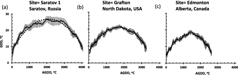
Figure 4. Fitted (dotted lines) average GDD as a function of AGDD superimposed with two standard error GDD error bars (gray crosses) for three croplands for 2003–2010. The coefficients of determination for Saratov 1, Grafton, and Edmonton are 0.96, 0.98, and 0.97, respectively. Interannual variability in GDD tended to be greater in the transitional seasons of spring and fall than in summer. Note the higher interannual uncertainty at the Russian site.
Download figure:
Standard image High-resolution image3.2. Vegetation optical depth
The behaviors of VOD as a function of AGDD exhibit distinct LSPs. During the growing season, VODs ascend to a unimodal peak value and then decline gradually. Peak VOD in the USA and Canada croplands occurred in early August for both frequencies on average. In contrast at the Russian sites the VOD peaks significantly earlier in mid-June (figure 5, table 2). VOD time series showed steep slopes towards their annual peak and then descended gently. The shapes of these seasonal trajectories may reflect microwaves' sensitivity to the timing of vegetation biomass growth and associated changes in canopy water content and the later season drydown and harvest. The pace of fractional green vegetation cover development is quicker than during its disappearance. TTPVOD differences between the AMSR-E two frequencies, 10.65 and 18.7 GHz, was notably higher for Winnipeg (316 AGDD ° C) (table 2).
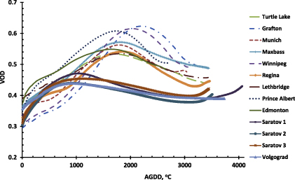
Figure 5. Interannual average (2003–2010) of vegetation optical depth (VOD) as a function of AGDD at the highest AMSR-E frequency. Croplands in Russia attained their peak VOD much earlier than that of the USA and Canada, but with a lower peak and smaller dynamic range.
Download figure:
Standard image High-resolution imageThe fitted convex quadratic LSP models for every site for both frequencies showed high coefficients of determination (r2 > 0.90, figure 6, table 2). The Russian sites displayed lower peak VODs that occurred earlier; whereas, the North American sites displayed higher VOD peaks that occurred at higher AGDD (figures 5 and 6, table 2). At each study site the VOD peak at the higher frequency (18.7 GHz) was higher than the VOD peak at the lower frequency (10.65 GHz), with the exception of the Prince Albert site, where the peaks were equal in magnitude (table 2). This pattern accords with the fact that the shorter wavelengths are more attenuated by the vegetation canopy and, thus, register higher VOD.
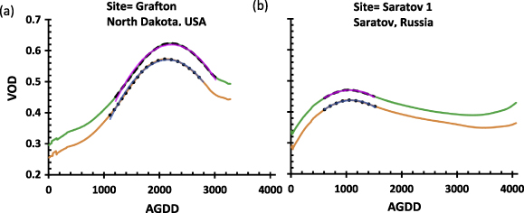
Figure 6. Convex quadratic land surface phenology models for VOD in USA (a) and Russia (b). Green is observed VOD at 18.7 GHz and orange is observed VOD at 10.65 GHz. Black dashed and dotted lines indicate the 'core growing season' used to fit each LSP model. The magenta line shows the fitted CxQ model of VOD at 18.7 GHz and the blue line shows the fitted CxQ model of VOD at 10.65 GHz.
Download figure:
Standard image High-resolution image4. Discussion
4.1. VOD and crop type
Peak VOD in Russia occurs much earlier (mid-June) compared to that of the North America (early August) (figure 5, table 2). The North American sites were planted to spring wheat that matures in the first half of August; whereas, the Russian sites were planted to winter grains and some grasses that grow and mature soon after the end of frozen season. Major crops that covered the Volgograd site include winter wheat, while the three Saratov sites were covered by winter wheat and some spring wheat. According to USDA Foreign Agricultural Service (FAS), each of these Russian sites was within the five major winter wheat producing oblasts that produce more than 60% of the Russian winter wheat crop (USDA FAS 2009). The USDA FAS also indicates that these Russian sites had minimal cover in rye (USDA FAS 2005). The North America croplands had longer growing season and much higher VOD peaks while the Russia croplands exhibited shorter growing season and lower peak VODs. While the difference in peak VOD timing results from phenological differences in winter versus spring grains, the magnitude of the VOD peak suggests differences in cultivation practices and grain varieties as well.
4.2. VOD and land cover
Some cropland sites show distinctive VOD trajectories. For example, the Edmonton site exhibited higher VOD much earlier in the season compared to other Canadian sites. Land cover information, gleaned from MODIS MCD12C1 IGBP 0.05° LC Type 1 percentage, indicates that ∼16% of the Edmonton study site falls within suburbs of Edmonton. The earlier season VOD may then result from woods, lawns, parks, and cemeteries in the suburban areas. Other sites having an urbanized component include Winnipeg and Volgograd (∼12% each). A study conducted in eastern North America using MODIS NDVI found the effects of urbanized areas on land surface phenology to decay exponentially from the urban boundary to 10 km into rural land covers (Zhang et al 2004). Vegetation in urbanized areas can experience longer growing season and lower canopy density compared to those in rural areas, i.e., they have earlier green-up and later dormancy (White et al 2002, Zhang et al 2004).
4.3. VOD, GDD, and the 2010 Russian heat wave
The effects of the 2010 Russian heat wave (Trenberth and Fasullo 2012) were evident in the AMSR-E time series. At the three Saratov sites, the GDDs were well above the expectation based on the 2003–2009 period, especially at Saratov 1 (figure 7(a)). The VODs were below expectation for much of the growing season as croplands were negatively impacted by the heat wave (Grumm 2011). Curiously, the VOD trajectory at Saratov 1 was closer to expectation than the other two sites that experienced more modestly elevated temperatures. At two Canadian sites at comparable latitude, the thermal regime was substantially lower than expectation (figure 7(c)). The VODs were significantly depressed at one location (Regina) but not the other (figure 7(d)), despite comparable thermal regimes (figure 7(c)), suggesting that factors other than the temperature affected the Regina LSP. The third Canadian site at the same latitude, Winnipeg, was not included in the comparison due to the influence of (sub)urban land uses within the AMSR-E pixel.
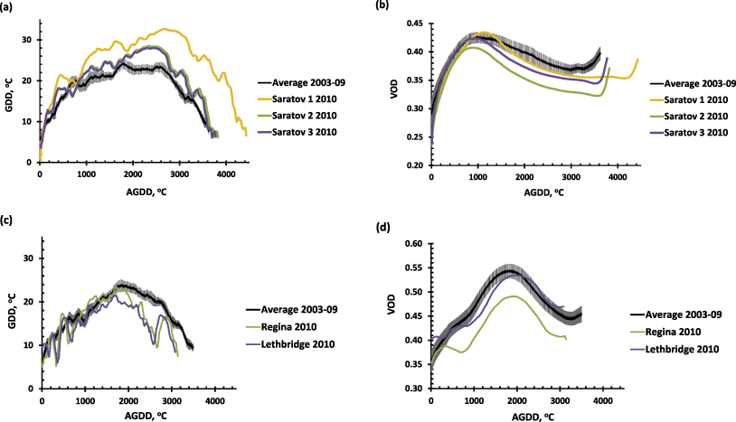
Figure 7. GDD and VOD as a function of AGDD reveal the impact of the 2010 Russian heat wave. The average values are bounded by two standard errors. Saratov 1, 2 and 3 time series show that GDDs were higher in 2010 (a), while the VODs were lower (b). Note the late season upswing in VOD results from fall planting of winter grains. The Regina and Lethbridge sites in Canada, at roughly the same latitude as Saratov, show thermal regimes cooler than expected, especially in the second half of the growing season (c). The VOD trajectory during green-up was significantly below expectation in Lethbridge but recovered during the later season (d). In contrast, at Regina the VOD trajectory was well below expectation (d), despite a similar sequence of GDDs (c). Other factors must account for the depressed VOD trajectory in Regina.
Download figure:
Standard image High-resolution image4.4. VOD compared to NDVI and meteorological station temperature data
Time series analysis of NDVI from Aqua MODIS (calculated from 8-day reflectance) and VOD from AMSR-E (8-day retrospective moving average) for the Saratov 1 site in Russia showed similar LSPs (figure 8). Both indicators of the vegetated land surface displayed correspondence with temperature data from a nearby meteorological station. The peak in the VOD time series lagged those in the NDVI. This behavior was expected since the VOD is sensitive to canopy water content; whereas, the NDVI is sensitive to photosynthetically active radiation (PAR) absorption (Viña et al 2004). Noise in the NDVI time series likely resulted from atmospheric effects, such as sub-pixel cloud contamination. While the NDVI displayed a higher dynamic range than the VOD, the late season secondary peak in winter grains is captured more consistently by the VOD than the NDVI (figure 8). Note how the dynamics in 2010 differ from the earlier years, particularly the long decline in VOD.

Figure 8. Time series plots of the VOD (cyan circles) and the NDVI (black circles) (2003–2010) from a single AMSR-E pixel, Saratov 1, in Russia. Temperature data (temp.ms) from a nearby meteorological station (red line) is superimposed. The station and VOD data were smoothed with an 8-day retrospective moving average. These data were aligned to the Aqua MODIS MYD09A1 reflectance compositing periods for comparison. All annual data (1 January–31 December) were considered. Notice that the seasonal bimodality of VOD is more pronounced than in the NDVI. The bimodality arises from the planting of winter grains in the fall, and growth and harvest in the subsequent early summer.
Download figure:
Standard image High-resolution image
An important limitation of the microwave data is its relatively coarse spatial resolution necessitated by the earth's surface low microwave energy emissions, limiting its ability to detect fine spatial scale changes (Liu et al 2011, 2013, Jones et al 2012). At the same time, the higher temporal resolution of the microwave data offers different insights in the land surface dynamics. Particularly useful is the retrieval of air temperature (rather than skin temperature) at much fine spatial resolution than ground-based meteorological station networks over most of the planetary land surface (although these temperature retrievals are limited in temporal resolution). Although the VOD retrievals span a very large area—nominally 625 km2—the sensitivity to the water content in the vegetated land surface offers a different perspective that may be more temporally responsive to root-zone soil moisture changes than the absorption of PAR which the NDVI indicates. Additional research is needed to investigate how best to use these complementary perspectives for monitoring and modeling the dynamics of the vegetated land surface.
5. Conclusion
Land surface phenologies (LSPs) of VODs and land surface seasonalities (LSSs) of GDDs based on times series of the AMSR-E enhanced land parameters followed seasonal patterns expected from thermally limited croplands. Both the microwave retrieved GDDs and VODs could be well fit using the convex quadratic land surface phenology (CxQ LSP) model that has been successfully applied in many biomes using optical data. The AMSR-E data were also able to detect the impact of the severe heat wave that devastated Russian crops in the summer of 2010. These results show the potential for passive microwave data in general and the AMSR-E enhanced land parameters in particular to be used for modeling cropland dynamics and, possibly, for forecasting agricultural productivity in data sparse regions of the world.
Despite the loss of the AMSR-E, there is a future for information from passive microwave land surface products. The Advanced Microwave Scanning Radiometer 2 (AMSR-2) onboard the Global Change Observations Mission 1st-Water (GCOM-W1), recently renamed SHIZUKU, was successfully launched by Japan Aerospace Exploration Agency (JAXA) in May 2012 and data products were released to the public in May 2013 (https://gcom-w1.jaxa.jp/). AMSR-2 has similar functions with AMSR-E, but with some improvements. The NTSG plans to continue the production of the enhanced land parameters using AMSR-2 datastreams (Kimball 2013). Extending this data record is an important step towards harnessing the power of passive microwave remote sensing for monitoring and modeling landscape dynamics beyond freeze–thaw transitions.
Acknowledgments
This research was supported in part by NASA grants NNX11AB77G and NNX13AN58G. The AMSR-E data were accessed from Numerical Terradynamic Simulation Group (NTSG) website (www.ntsg.umt.edu/project/amsrelp). The MODIS MYD09A1 data were obtained from the Oak Ridge National Laboratory Distributed Active Archive Center (http://daac.ornl.gov/cgi-bin/MODIS/GLBVIZ_1_Glb/modis_subset_order_global_col5.pl). The meteorological data were acquired from NOAA National Climatic Data Center website (http://gis.ncdc.noaa.gov/map/viewer/#app=cdo&cfg=cdo&theme=temp&layers=1). We gratefully acknowledge the thoughtful comments from two anonymous reviewers that increased the clarity of the presentation.