
Abstract
The existence of a meteorological response in the polar regions to fluctuations in the interplanetary magnetic field (IMF) component By is well established. More controversially, there is evidence to suggest that this Sun–weather coupling occurs via the global atmospheric electric circuit. Consequently, it has been assumed that the effect is maximized at high latitudes and is negligible at low and mid-latitudes, because the perturbation by the IMF is concentrated in the polar regions. We demonstrate a previously unrecognized influence of the IMF By on mid-latitude surface pressure. The difference between the mean surface pressures during times of high positive and high negative IMF By possesses a statistically significant mid-latitude wave structure similar to atmospheric Rossby waves. Our results show that a mechanism that is known to produce atmospheric responses to the IMF in the polar regions is also able to modulate pre-existing weather patterns at mid-latitudes. We suggest the mechanism for this from conventional meteorology. The amplitude of the effect is comparable to typical initial analysis uncertainties in ensemble numerical weather prediction. Thus, a relatively localized small-amplitude solar influence on the upper atmosphere could have an important effect, via the nonlinear evolution of atmospheric dynamics, on critical atmospheric processes.
Export citation and abstract BibTeX RIS

Content from this work may be used under the terms of the Creative Commons Attribution 3.0 licence. Any further distribution of this work must maintain attribution to the author(s) and the title of the work, journal citation and DOI.
Corrections were made to this article on 16 October 2013. A corrected version of the supplementary material was uploaded.
1. Introduction
Meteorological effects resulting from fluctuations in the solar wind are presently poorly represented in weather and climate models. Indeed, the role of the Sun is one of the largest unknowns in the climate system [1]. The existence of a meteorological response in the polar regions to fluctuations in the dawn–dusk component of the interplanetary magnetic field (IMF), By, is well established [2–5] and is known as the 'Mansurov effect'. More controversially, there is evidence to suggest that this Sun–weather coupling occurs via the global atmospheric electric circuit [4, 5]. Consequently it has been assumed [6] that the effect maximizes at high latitudes and is negligible at low and mid-latitudes because the perturbation by the IMF is concentrated in the polar regions [7, 8]. However, the spatial variation of the IMF-weather coupling has not been investigated over the whole globe.
In the most detailed study to date [5], variations in IMF By of ∼8 nT were associated with changes in high-latitude station surface pressure of ∼1–2 hPa. These correlations were statistically significant for Antarctica between 1995 and 2005, and in the Arctic between 1999 and 2002. The time lag between changes in IMF By and changes in the surface pressure was estimated to be approximately 0 ± 2 days. Here we extend the analysis, for zero time lag, using 12 UT NCEP/NCAR reanalysis surface pressure [9] data on a global grid (λ,ϕ) where λ is latitude and ϕ is longitude (section 2). A similar spatial analysis of the ionospheric potential for different states of IMF By (section 3) is used to investigate the theory that the response of surface pressure to fluctuations in IMF By occurs via the global atmospheric electric circuit. Our results indicate that a mechanism that is known to produce atmospheric responses to the IMF in the polar regions is also able to modulate weather patterns at mid-latitudes.
2. Surface pressure ordered by IMF By
For the interval 1999–2002, when statistically significant correlations were seen in both the Arctic and in Antarctica [5], we remove the seasonal cycle. The seasonal cycle is approximated by the mean 12 UT value for each 'day of year' on the model latitude and longitude grid (λ,ϕ) using 1948–2011 data. We then determine the mean of the residual surface pressures for high positive IMF By (≥3 nT), high negative By (≤−3 nT), and all By, in the geocentric solar magnetospheric (GSM) coordinate system, where positive By is aligned from dawn to dusk. We denote these quantities by  (figures S1(a)–(d) in the supplementary data, available at stacks.iop.org/ERL/8/045001/mmedia) and
  , respectively; the zonal averages are denoted by
  ,
,  , and
, and  . The ordering of surface pressure by IMF By and by hemisphere (the Mansurov effect) is evident in figures 1(a) and (b) in the anomalies
  ,
,  and in the quantity

where 'O' stands for 'ordered by IMF By'. At low latitudes (∼38° S–48° N),  and
and  are generally not distinct, only becoming so at mid- to high-latitudes. The amplitude of
  is larger in the southern than in the northern polar regions as previously noted [5]. The greatest difference between
  and
and  occurs at ∼80° S, in Antarctica. Poleward of ∼58° S,
  exceeds
  , whilst poleward of ∼50° N the situation is reversed:
  exceeds
  . We conducted a Wilcoxon Rank-Sum (WRS) test between
  and
and  (figure 1(c)). This is a non-parametric test of the null hypothesis that these two populations of pressure measurements have the same mean of distribution, against the hypothesis that they differ. Poleward of 58° S and 50° N,
  and
and  differ with very high statistical significance (below the 1% level). This is also the case for limited intervals between 58° S and 50° N. Further details of the method are in section 1 of the supplementary data (available at stacks.iop.org/ERL/8/045001/mmedia).

Figure 1. The zonal mean surface pressure depends on IMF By at mid- to high-latitudes. (a) The latitudinal profiles  and
and  , shown in red and blue respectively, are ordered by IMF By and by hemisphere. (b)
  , the difference between the red and blue lines in (a), is ordered by hemisphere. (a) and (b) Error bars indicate the error in the mean. (c) The one-tailed probability of obtaining the Z value from a WRS test between
  (the average over 50 688 datapoints) and
  (39 312 datapoints) shows that
  and
and  are most significantly different for latitudes poleward of 50°–60°.
Download figure:
Standard image High-resolution imageWe now consider the two-dimensional (2D) surface pressure. The 1999–2002 average,  (figures 2(a) and (b)), shows that an m = 3 quasi-stationary atmospheric Rossby wave [10, 11], with three wavelengths circumnavigating the globe, is a dominant wave mode in the Southern Hemisphere (see also figure S2(c) and section 2 of the supplementary data, available at stacks.iop.org/ERL/8/045001/mmedia). The dominant wave mode in the Northern Hemisphere is not so clear but has an m = 5 component (figure S2(a), available at stacks.iop.org/ERL/8/045001/mmedia). The difference between the mean surface pressures for times of high positive and high negative IMF By is:

 is positive in Antarctica and predominantly negative in the Arctic (figures 2(c) and (d)), as previously noted for this interval [5], with an amplitude comparable to those previous observations. What has not been shown before is that, although the zonally-averaged difference
  at mid-latitudes is well below that at high latitudes (figure 1(b)), the amplitude of the 2D field
  over much of the mid-latitude region is comparable to that at high latitudes. This is because at mid-latitudes
  possesses a wave structure that is reminiscent in location and form to atmospheric Rossby waves (figures S2(b) and (d), available at stacks.iop.org/ERL/8/045001/mmedia).
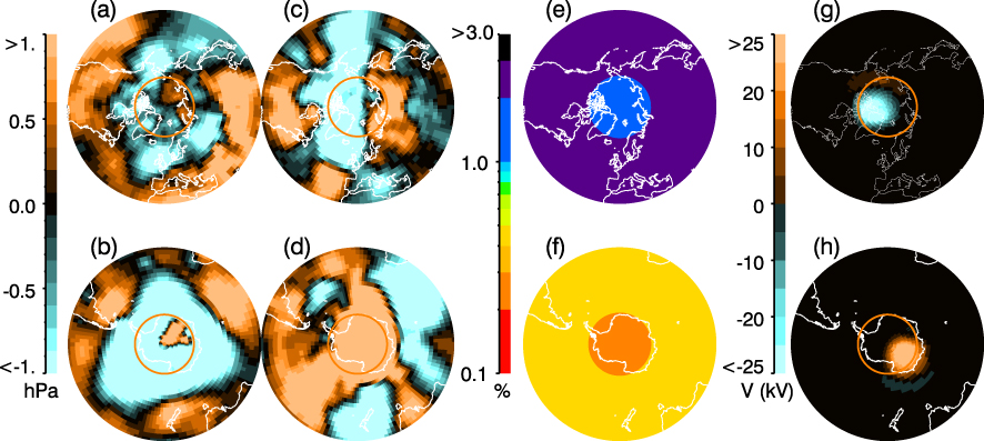
Figure 2. (a) and (b) The 1999–2002 average of the surface pressure,  , has a clear m = 3 quasi-stationary Rossby wave in the Southern Hemisphere. (c) and (d) The difference between IMF By high and positive and By high and negative,
  : the amplitude at mid-latitudes is comparable to that at high latitudes. (e) and (f) The WRS test between
  (352 datapoints) and
  (273 points) has most field significance in the Southern Hemisphere at high and mid-latitudes (both at <0.5%), but field significance is high (at <5%) for all regions except 'Equatorial' (see table 1 and figure S1, available at stacks.iop.org/ERL/8/045001/mmedia). (g) and (h) The spatial dependence and polarity of
  (4), is similar in form to
  at high latitudes. This supports the hypothesis that surface pressure is influenced by IMF By via the global atmospheric electric circuit. (a)–(h) The lowest latitude is λ = 30°; orange circles mark λ = 70°.
Download figure:
Standard image High-resolution imageAt each grid point (λ,ϕ) we conducted a WRS test between  and
and  . We evaluate the resulting 2D grid of significance values in a way that corrects for the 'false discovery rate' over a region (the expected fraction of local null hypothesis rejections that are actually true [12]). The resulting 'field significance' calculations for each of five different regions and for the whole globe are listed in table 1 and plotted in figures 2(e), (f) and S1(g), (h) (available at stacks.iop.org/ERL/8/045001/mmedia). The difference between
  and
and  is highly statistically significant (below 5%) globally and in all examined regions except for the 'Equatorial' region. There are higher levels of statistical significance in the southern mid- and high-latitudes than in the corresponding regions in the Northern Hemisphere.
Table 1.
Field significances for WRS test between  and
and  .
.
| Region | Latitude range (deg) | Field significance (%) |
|---|---|---|
| Arctic | 70.0N–90.0N | 1.90 |
| Mid-latitude (north) | 30.0N–70.0N | 2.06 |
| Equatorial | 30.0S–30.0N | 23.5 |
| Mid-latitude (south) | 30.0S–70.0S | 0.44 |
| Antarctica | 70.0S–90.0S | 0.26 |
| Globe | 90.0S–90.0N | 2.01 |
The same zonal and 2D analyses conducted using sea-level pressure give similar results (figures S3 and S4, and table S1, available at stacks.iop.org/ERL/8/045001/mmedia). The significance of the  field was also investigated using the joint Shannon entropy [13], and the results confirm that IMF By is associated with a statistically significant change to the surface pressure field at mid- and high-latitudes (figures S6 and S7, and section 3 in the supplementary data, available at stacks.iop.org/ERL/8/045001/mmedia).
3. Evidence for action via the global atmospheric electric circuit
The electric potential difference V between the ionosphere and the Earth's surface can be decomposed into two components [6]:

The first term Va is driven by thunderstorms distributed around the globe that sustain a potential difference of ∼250 kV between the ground and ionosphere [14]. The second term Vi is driven by the solar wind which continually interacts with Earth's magnetosphere via magnetic reconnection, driving the transport of plasma through the magnetosphere. This results in a dawn-to-dusk potential difference across the high-latitude polar cap ionosphere that depends on the IMF magnitude and direction [15]. The spatial variation of the solar-wind-driven ionospheric potential Vi is well understood [7, 8]. Figures S8(a)–(d) (available at stacks.iop.org/ERL/8/045001/mmedia) show its average configuration in corrected geomagnetic (CGM) coordinates for predominantly dawnward (By < 0) and predominantly duskward (By > 0) directed IMF for 5 < |B| < 10 nT. Taking the time-averaged difference of the vertical potential difference (3) between these two By configurations, we eliminate the potential Va due to the atmospheric thunderstorm-generated electric field which we assume to be independent of B to obtain:

where  corresponds to the By > 0 configuration and
  corresponds to the By < 0 configuration.
  is approximately circularly symmetric about the geomagnetic pole, negative poleward of ∼74° N CGM latitude, positive poleward of ∼74° S CGM, and small elsewhere (figures S8(e) and (f), available at stacks.iop.org/ERL/8/045001/mmedia).
  is plotted in geographic coordinates in figures 2(g) and (h). The asymmetry with hemisphere in the polarity of
  at high latitudes is the same as that found in
  in this region, shown in figures 2(c) and (d). Therefore we propose that it is changes in the ionospheric electric potential field, driven by changes in the IMF By component, that directly affect the surface atmospheric pressure at high latitudes, although the full details of the mechanism are presently unknown. Future studies, for instance of seasonal dependence, may help to pinpoint the mechanism. It should be noted that some observations of a solar wind modulation of lightning have been made [16] but the conclusions of different studies are contradictory.
4. Discussion and conclusions
To explain the observed correlation of IMF By with surface pressure we propose that the mid-latitude surface pressure is influenced by IMF By via a two-stage process comprising: (i) a change in the polar surface pressure involving the global atmospheric electric circuit [5, 6], and (ii) a resulting change in the mid-latitude surface pressure via conventional meteorology. The first of these two processes, concerning the influence of IMF By fluctuations on the polar surface pressure remains under-explored and controversial [17, 18]. However, our analysis of the surface pressure anomaly field  provides new evidence supporting a direct relationship with the ionospheric electric potential.
Figure 3 is a schematic representing this two-stage process: in the Northern Hemisphere, as IMF By switches from dawnward to duskward, the potential difference between the ionosphere and the Earth's surface, V, and the sea-level pressure p, decrease in the northern polar region. The direct effect on sea-level pressure in the polar regions (figures S3 and S4, available at stacks.iop.org/ERL/8/045001/mmedia), along with the lack of effect on pressure at low latitudes, results in a change in the latitudinal sea-level pressure gradient in mid-latitude regions (figure S5, available at stacks.iop.org/ERL/8/045001/mmedia) associated with an increase in the mean zonal wind U at mid-latitudes. Generalizing the original theory of Rossby waves [10] to the case of periodic variations in both longitude and latitude [19], we obtain U = β/(k2 + l2) where k and l are the wavenumbers in the longitudinal and latitudinal directions, respectively. For a fixed value of k (and hence m), an increase in U leads to a decrease in l and an increase in meridional wavelength Lθ. Thus variations in IMF By modify the quasi-stationary Rossby wavenumber (k,l), accounting for the Rossby-wave-like form of  . The variations in V,p,U,l and Lθ are reversed in the Southern Hemisphere. More details are in section 2 of the supplementary data (available at stacks.iop.org/ERL/8/045001/mmedia).

Figure 3. Our hypothesis is that the mid-latitude surface pressure is influenced by IMF By via a two-stage process. (i) As IMF By changes from dawnward to duskward, the electric potential difference between the ionosphere and the Earth's surface, V, and the sea-level pressure p, decrease in the northern polar region; (ii) the mean zonal wind U at mid-latitudes increases resulting in an increase in the meridional wavelength (for simplicity labelled L in this figure; in text referred to as Lθ) of the stationary Rossby wave with an integer number of azimuthal waves m (at co-latitude θ and latitude λ = 90° − θ). The variations in V,p,U and L are reversed in the Southern Hemisphere.
Download figure:
Standard image High-resolution image
Previously, proposals to link solar wind variations to significant weather or climate variability have been dismissed on the grounds that the magnitude of the energy change in the atmosphere associated with the solar wind variability is far too small to impact the Earth's system. However, this argument neglects the importance of nonlinear atmospheric dynamics [20]. The amplitudes of the IMF-related changes in atmospheric pressure gradient are comparable with the initial uncertainties in the corresponding zonal wind used in ensemble numerical weather prediction (NWP) [21] of ∼1 m s−1. Such uncertainties are known to be important to subsequent atmospheric evolution and forecasting [22]. Consequently, we have shown that a relatively localized and small-amplitude solar influence on the upper polar atmosphere could have an important effect, via the nonlinear evolution of atmospheric dynamics on critical processes such as European climate and the breakup of Arctic sea ice [23].
In particular, it affects the structure of the Rossby wavefield, which is key in determining the trajectory of storm tracks [24]. The configuration of the North Atlantic jet stream is particularly susceptible to changes in forcing [25]. In turn, so are the location and the timing of blocking events in this region, in which vortices are shed from the jet stream leading to prolonged periods of low or of high pressure [26]. It has also been proposed that the low-frequency variability of the North Atlantic Oscillation (NAO) arises as a result of variations in the occurrence of upper-level Rossby wavebreaking events over the North Atlantic [27]. The NAO itself is key to climate variability over the Atlantic–European sector stretching from the east coast of the United States to Siberia, and the Arctic to the subtropical Atlantic [28, 25].
Our results may therefore provide part of the explanation for previously observed correlations between Eurasian winter temperatures and solar variability [29, 30], and for the 'Wilcox effect' where reductions in the areas of high vorticity in winter storms are seen at times of solar wind heliospheric current sheet crossings [31] (which are characterized by sharp changes between steady, opposite IMF By states).
Acknowledgments
NCEP Reanalysis data were provided by the NOAA/OAR/ESRL PSD, Boulder, Colorado, USA, from their website www.esrl.noaa.gov/psd/. The OMNI data were obtained from the GSFC/SPDF OMNIWeb interface at http://omniweb.gsfc.nasa.gov. We thank Christian Franzke (British Antarctic Survey) for introducing us to global field significance testing and Cosma Shalizi (Carnegie Mellon University) for discussions on entropy. The software used to produce plots of ionospheric potential was written and kindly provided by Ellen Cousins (nee Pettigrew) at the High Altitude Observatory (NCAR), Boulder, Colorado. The authors acknowledge support by the UK Natural Environmental Research Council (NERC) grant NE/I024852/1.