
Abstract
Increasing demand for crop-based biofuels, in addition to other human drivers of land use, induces direct and indirect land use changes (LUC). Our system dynamics tool is intended to complement existing LUC modeling approaches and to improve the understanding of global LUC drivers and dynamics by allowing examination of global LUC under diverse scenarios and varying model assumptions. We report on a small subset of such analyses. This model provides insights into the drivers and dynamic interactions of LUC (e.g., dietary choices and biofuel policy) and is not intended to assert improvement in numerical results relative to other works.
Demand for food commodities are mostly met in high food and high crop-based biofuel demand scenarios, but cropland must expand substantially. Meeting roughly 25% of global transportation fuel demand by 2050 with biofuels requires >2 times the land used to meet food demands under a presumed 40% increase in per capita food demand. In comparison, the high food demand scenario requires greater pastureland for meat production, leading to larger overall expansion into forest and grassland. Our results indicate that, in all scenarios, there is a potential for supply shortfalls, and associated upward pressure on prices, of food commodities requiring higher land use intensity (e.g., beef) which biofuels could exacerbate.
Export citation and abstract BibTeX RIS

Content from this work may be used under the terms of the Creative Commons Attribution-NonCommercial-ShareAlike 3.0 licence. Any further distribution of this work must maintain attribution to the author(s) and the title of the work, journal citation and DOI.
1. Introduction
Biofuel production has been pursued because of opportunities to contribute to climate change mitigation, among other potential benefits such as securing and diversifying energy supply and providing, economic development opportunities especially in rural areas. Initial biofuel assessments (e.g., Farrell et al 2006) suggested that biofuels, such as corn ethanol, could help the United States (US) reduce greenhouse gas (GHG) emissions. However, Searchinger et al (2008) and Fargione et al (2008) highlighted that previous biofuel studies failed to include the effects of global land use change (LUC). These two watershed studies modeled the potential impact of carbon released from soils and above-ground biomass during land clearing activities triggered by increased demand for biofuel. Results from these studies, as well as many other biofuel-induced LUC studies (e.g., see Berndes et al 2010), hinge on assumptions regarding direct and indirect causal relationships (see section 1 of the supplemental information (SI), available at stacks.iop.org/ERL/8/015003/mmedia, for more detail) between drivers of LUC, land availability, biomass yields, population dynamics, dietary choices, relative affluence, and biofuel demand, to name a few. However, the causal relationships that underpin such results are not completely understood and there remains significant disagreement on many fundamental aspects of LUC dynamics. LUC, as well as those changes attributable to biofuels, has far-reaching implications for many aspects of sustainability i.e., biodiversity and societal impacts (e.g., food security). For example, diversion of land to biofuel crops displaces production that may lead to compensating production of substitute crops elsewhere, affecting regional food crop prices (Chum et al 2011, Dale et al 2011). Therefore, a better understanding of the drivers of LUC and high-level influences on system behavior is critical to the responsible and sustainable development of biofuels.
Inclusion of LUC impacts in renewable fuels policy is contentious, because it is neither directly measurable nor easily isolated from the myriad of other LUC drivers (Plevin et al 2010), such as agricultural policies, agricultural product demand changes, and social norms. Biofuel policy analyses typically rely on computer simulations or on extrapolations of historic data to evaluate total LUC. The LUC modeling science lacks consensus with regard to modeling frameworks, boundary conditions, and other fundamental assumptions, which has resulted in highly variable modeling results across a wide range of studies. For example, results of CO2 emissions from biofuel-induced LUC span an order of magnitude, and subsequent calculations of GHG emissions can even vary in sign (Berndes et al 2010). Currently, US and European governmental organizations are integrating—or are considering integrating—LUC impacts into their renewable fuel policies (e.g., the US Renewable Fuel Standard (RFS) US EPA 2010), EU Renewable Energy and Fuel Quality Directive (European Commission 2009), United Kingdom (UK) Renewable Transport Fuel Obligation (Gallagher 2008, UK Department for Transport 2012), and California's Low Carbon Fuel Standard (CARB 2009). At present, analysts often use agricultural economic models. For example, variations of the Global Trade Analysis Project (GTAP) database and the US EPA's methodologies are commonly being used to estimate GHGLUC for renewable fuel policy purposes (US EPA 2010, Tyner et al 2010, Al-Riffai et al 2010).
The modeling approach presented in this study is intended to complement existing approaches and to improve the understanding of global LUC drivers and dynamics. Every effort has been made to ensure the model is parsimonious and transparent, both in terms of the underlying data and the feedback effects among drivers. By using a model with high transparency, ease of use, and dynamic capabilities, our study improves policy-relevant analyses by allowing examination of global LUC under diverse scenarios and varying model assumptions. In this paper, we report on a small subset of such analyses. These are intended as an initial illustration of model functionality, not to assert improvement in numerical results relative to other work.
2. LUC models and approaches
Based on our review of the literature, we categorize most biofuel-related LUC modeling approaches into three broad categories: (1) general and partial economic equilibrium modeling, (2) simple deterministic methods, and (3) causal descriptive methods. Each method has strengths and weakness in modeling LUC and its causes (see table 1), because purposes of models vary. Modeling classifications listed in table 1 suggest a spectrum of complexity, with higher complexity on the left side.
Table 1. Comparison of models using different methods used to estimate LUC in existing literature (Ackerman 2002, ICF International 2009, CBES 2009). Specific models may differ from these generalizations.
| General and partial economic equilibrium models | System dynamics | Causal descriptive method | Deterministic method (simplified) | |
|---|---|---|---|---|
| Description | Calculates LUC resulting from the cause-and-effect relationships in a market system based on the change resulting from shocking an economic system at equilibrium with an expansion of biofuels. Uses historic data for calibration, but may incorporate empirically estimated functions. Model parameters are often derived from related literature | Calculates LUC using cause-and-effect relationships in a dynamic stock-and-flow framework to assess market responses resulting from increasing demand for biofuels. Uses historic trends as inputs and for calibrating cause-and-effect relationships | Calculates LUC using cause-and-effect relationships to assess market responses resulting from increasing demand for biofuels. Uses historic trends as inputs and for calibrating cause-and-effect relationships | Generates an 'average' adder for agricultural products considered relevant to the bioenergy sector based on historic land use data. Direct and indirect LUC are sometimes combined but sometimes separate factors |
| Potentially limiting assumptions in existing models | (1) LUC is driven primarily by price-related economic forces. (2) Non-price factors are assumed to be exogenous and generally held constant | (1) Future market responses (e.g., product substitution, cultivation area of a given crop) to increased demand for biofuels can be extrapolated from historical trends and relationships between economic, agricultural, and social systems. (2) Market responses are driven by relatively independent external assumptions, but internal moderating feedbacks are included | (1) Future market responses (e.g., product substitution, cultivation area of a given crop) to increased demand for biofuels can be extrapolated from statistical analysis of historical trends. (2) Market responses are relatively independent and can be quantified without considering possible correlations | (1) Only countries trading evaluated agricultural commodities might be subject to LUC effects. (2) The patterns of global trade of agricultural commodities will remain virtually unchanged in the near future, and therefore the incremental effect of biofuel expansion on land use will always have the same global impact. (3) LUC caused by increased biofuel feedstock production can be directly estimated from the type and share of land used to grow agricultural commodities for export purpose |
| Strengths | (1) Captures, in detail, many important market and economic factors that can drive LUC. (2) Usually based at institutions that offers technical support. (3) In its dynamic form can account for the evolution of demographic variables and resources, and other changes over time | (1) Can relatively easily incorporate important LUC drivers other than market and economic factors. (2) Can be transparent and involve stakeholders in running the model and scenario development | (1) Can relatively easily incorporate important LUC drivers other than market and economic factors. (2) Can be transparent and involve stakeholders in running the model and scenario development | (1) Easy to calculate and transparent |
| Limitations | (1) Currently, usually fails to include other important LUC drivers (e.g., political, cultural, demographic, environmental forces) that may not rely on land and commodity prices and elasticities. (2) Difficult to gain access to or use by non-experts economic modelers | (1) Misses dynamic and interlinked LUC driving factors in cause-and-effect chains because of reliance on historical data and relationships to identify LUC drivers. (2) Data and relationships operate at a relatively aggregate low-resolution level. (3) Prices need not be explicitly modeled | (1) Misses dynamic and interlinked LUC driving factors in cause-and-effect chains because of reliance on historical data and relationships to identify LUC drivers. (2) Data and relationships operate at a relatively aggregate low-resolution level. (3) Prices need not be explicitly modeled | (1) Generally does not consider land types not used for producing traded agricultural commodities. (2) Omits market feedbacks and policy measures that affect trade patterns. (3) Data and relationships operate at a very aggregate low-resolution level |
| Example papers | Hiederer et al (2010), Al-Riffai et al (2010), US EPA (2010), Tyner et al (2010), Wise et al (2009) | Sheehan (2009) | Bauen et al (2010), Lywood (2008) | Kim et al (2009), Fritsche et al (2010), Tipper et al (2009) |
The new model, called BioLUC, is a system dynamics (SD) simulation model (NREL 2012, Bush et al 2011) that represents key economic and social drivers of global LUC and their interactions over time, enabling exploration of different scenarios with implications for LUC5. In particular, BioLUC can explore implications of and assumptions about LUC by analyzing the limits of sustainable biofuels production under varied future conditions regarding inputs, specifically population growth, crop yields, and plant and animal product supply and demand. BioLUC was created using the STELLA Version 9.1.4 software package (ISEE Systems, Lebanon, NH) using a stock-and-flow structure; it focuses on information feedback processes that underwrite the dynamic movement of key quantities over time.
BioLUC generally would fit the causal descriptive category. However, to-date, causal descriptive modeling systems have been spreadsheet-based models that lack dynamic stock-and-flow frameworks. To explain the distinctions we describe SD models in a separate column in table 1. See section 2 of the SI (available at stacks.iop.org/ERL/8/015003/mmedia) for additional details about SD modeling, its historical context, and its use in projecting the consequences of today's and potential future policies.
The BioLUC model recognizes the accomplishments of past LUC modeling efforts and provides a modeling option that may address some of the limitations of current methods evaluating LUC and complement and existing suite of models to improve research insights. Transparency and ease of use are challenging to achieve when examining issues of biofuel-induced LUC, especially for the many interested stakeholders who are not economic modeling specialists. Enabling this community to access a transparent analytic method can help them work together to understand and analyze underlying LUC drivers; test assumptions about LUC systems against historic data; investigate future conditions; and assess implications of new LUC research results (Sheehan 2009, 2012). As tools for this kind of shared exploration, existing models are either too complex, with light model structure documentation, difficult data access, or, alternatively, grossly simplistic (i.e., deterministic method). A SD modeling approach building on the causal descriptive method attempts to fill this analysis space.
3. BioLUC modeling approach
The generalized influence diagram for a generic region of the world in the BioLUC model is presented in figure 1. The movement of land between usage categories over time is represented in the model using stocks for four different land bases, which flows into or out of those stocks. Within the 'crops' land base, land is allocated among multiple competing uses (e.g., food, feed, fuel, and fiber). Note the 'abandoned' category among the land bases: this land category, assumed nonproductive, enables us to explore land abandonment and rehabilitation scenarios. 'Available' land is forest and grassland that is potentially available for productive use as pasture or cropland.
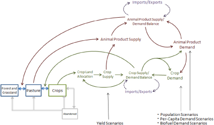
Figure 1. Illustrative influence diagram for each geographic regions modeled i.e. US and the rest of the world (ROW). Primary land stocks are represented by boxes, interactions are represented by connecting arrows, and inputs variables are represented by unboxed text.
Download figure:
Standard imageFigure 1 also shows how externally defined scenarios for key parameters impact the system: biomass yield and crop land allocation determine production of various crops; and population, per capita demand, and biofuel demand drives 'direct' demands for various crops.
BioLUC represents key feedback processes that drive the allocation of land over time. Examples of these processes include:
- Imbalances between production and consumption of various agricultural products motivate changes in the allocation of land among different uses at a regional level.
- Demand for animal products creates additional demand for crops grown as feed.
- Crop and animal product imbalances between production and consumption stimulate adaptive responses in the system to move toward equilibrium.
- Reallocation of existing crop land among different uses balances the mix of crops produced against the mix of crops required.
- Re-distribution of the land bases, for example by converting available land into pastureland or by turning pastureland into crop land, adjusts production to more closely meet demand.
- Crop or animal product imbalances are further reduced through imports/exports from other regions.
An imbalance between demand and supply stimulates multiple feedback mechanisms. For example, holding other things equal, if the combination of population, per capita demand, and biofuel scenarios cause consumption of a particular crop to exceed its production within a region several processes will begin to unfold:
- Regional inventories of the crop will begin to decline.
- The resulting supply shortfall will constrain consumption to levels lower than those implied by population, per capita demand and biofuel scenarios.
- The supply shortfall will cause the region to call for imports from outside the region, in the immediate term.
- Additionally, the supply shortfall will lead to a reallocation of crop land in favor of the crop in question in the longer term.
- Reallocation of cropland will increase the rate at which land moves from pasture into crops, which in turn will increase pressure to convert land from forest or grassland into pasture.
As these processes play out over time, the system will seek to balance itself so that equilibrium between supply and demand for crops within a region is restored.
We initially developed a two-region model that can be used to represent any two regions. See section 2 of the SI (available at stacks.iop.org/ERL/8/015003/mmedia) for more detail on two-region model structure and intra-regional trade. For additional details about model input assumptions including agricultural commodity yields, changes in population, and initial land cover at the start of the model across all scenarios, see data and model calculations in section 3 of the SI (available at stacks.iop.org/ERL/8/015003/mmedia).
4. BioLUC model scenarios
We explore four scenarios to broadly examine the effects of demand for crop-based biofuels and food on LUC as outlined below and in table 2. We constructed scenarios to represent an extreme high-intensity agricultural future to adequately highlight model dynamics and test model integrity under high pressures. The details of these scenarios are included in section 4 of the SI (available at stacks.iop.org/ERL/8/015003/mmedia), which describes biofuel yields, conversion yields, food and feed demand, and biofuel demand assumptions for several time steps of each scenario.
Table 2. BioLUC demand scenarios. The scenarios are modeled from 1990–2050. Input data is annual, but the model runs on a time step of 1/32nd of a year.
| Conditions in 2000 | • 9 million ha harvested for biofuels | |
| • 0.6 EJ biofuels | ||
| • 110–280 kg meat and dairy/capita-yr | ||
| • 260–300 kg other food/capita-yr | ||
| Lower biofuels demand | Higher biofuels demand | |
| Lower food demand | Business-as-usual (BAU) scenario | Higher biofuel (HB) scenario |
| By 2050: | By 2050: | |
| • 80 million ha harvested for biofuels | • 700 million ha harvested for biofuels | |
| • 7 EJ biofuels | • 46 EJ biofuels | |
| • 140–310 kg meat and dairy/capita-yr | • 140–310 kg meat and dairy/capita-yr | |
| • 280–290 kg other food/capita-yr | • 280–290 kg other food/capita-yr | |
| Higher food demand | Higher food (HF) scenario | Higher food and biofuel (HFB) scenario |
| By 2050: | By 2050: | |
| • 80 million ha harvested for biofuels | • 700 million ha harvested for biofuels | |
| • 7 EJ biofuels | • 46 EJ biofuels | |
| • 200–360 kg meat and dairy/capita-yr | • 200–360 kg meat and dairy/capita-yr | |
| • 330–340 kg other food/capita-yr | • 330–340 kg other food/capita-yr | |
The two crop-based biofuel demand levels are presumed to be policy driven rather than economically driven. The basis for setting the demand levels is as follows:
- (1)Lower biofuels demand is mostly based on levels and assumptions from Alexandratos and Bruinsma (2012), in which current (as of 2012) biofuels policies are met through increased use of food-based crops to 2020, with no subsequent growth. One adjustment made to Alexandratos and Bruinsma (2012) was the use of cellulosic ethanol starting in 2016 to meet ethanol requirements. Corn ethanol was effectively capped at the policy mandated level of 57 billion dm3 (15 billion gallons) (US EPA 2010).
- (2)Higher biofuels demand based on linear growth to reach a 25% global displacement of gasoline and diesel by 2050 using advanced (cellulosic and renewable diesel) biofuel systems, in addition to the biofuels in the lower biofuel demand scenario. Displacement of fossil fuels is calculated on an energy basis, with no petroleum market rebound effect.The two food and feed demand levels are:
- (3)Lower demand growth based on levels of per capita demand for food from Alexandratos and Bruinsma (2012).
- (4)Higher demand growth based on high-end demand projections (∼40% increases in per capita food demand by 2050 from 2005) were taken from Tilman et al (2011) and modified to be applied to the aforementioned projections from Alexandratos and Bruinsma (2012). Tilman et al (2011) does not specify how the demand increase is distributed across individual food categories. We closely approximate the ∼40% increase by equally applying changes across all commodities through a 45% increase in annual growth of each commodity demanded starting in 2010 relative to the low food demand scenario.
The four scenarios, presented in table 2, are limited in at least two key respects.
First, our examination of yield is constrained. FAO (2010) resolution is limited to national-level averages. In our high demand scenarios, we do not assume higher levels of agricultural intensification (i.e., higher than BAU yields increases) in response to economic forces, nor do we examine reductions in crop yields, as could result from climate change and increases in extreme weather events. Our yield data (from FAOSTAT) are aggregate national averages that can have large internal spatial and temporal variability. A limited scenario analysis examining the impact of higher and lower cellulosic biofuel yield trend assumptions was examined in section 6 of the SI (available at stacks.iop.org/ERL/8/015003/mmedia) and is discussed briefly in the results section, below.
Second, we model the high biofuels case essentially as higher land requirements to grow the biofuel feedstock on agricultural land (i.e., not wastes or residues or grown on marginal lands). We selected these limitations to test extreme land use conditions and to simplify the analyzed scenarios. The suite of feedstocks grown and technologies used is essentially generic: a shift in technology, feedstock, or yield assumption would only alter the aggregate land requirements (i.e., ∼700 million ha) examined in this analysis. The implications of these limitations will be discussed further in our results.
5. Results and discussion
BioLUC results are not predictions; the model only provides insights into the drivers and dynamic interactions of LUC. Quantities and changes are only provided to facilitate comparisons between our scenarios.
Business-as-usual (BAU) projections of LUC for the US and ROW are presented in figure 3. These results reflect changes in land use in response to global population growth and an overall increase in per capita gross domestic product, which causes diets to shift toward more calories per capita as well as a greater percentage of those calories coming from meat and animal products (e.g., dairy) (Alexandratos and Bruinsma 2012). Results suggest that the rate of conversion of available land (i.e., forest and grasslands) to cropland increases globally, relative to historic data in the US and the ROW, in order to meet rising food needs. In the ROW the rate of cropland increase remains similar to historic rates of change, but pastureland grows significantly. Pastureland trends in the ROW reflect the larger relative shift in per capita gross domestic product in developing countries. Land conversion begins to slow circa 2030 because the rate of population growth and per capita food demand growth begins to stabilize.
Globally, the most noticeable trend in the ROW is the increase in pastureland area to meet meat and animal product demands as the world's population grows and becomes more affluent. This is consistent with well-documented historic trends that show that increased wealth prompts a shift from diets rich in whole vegetables toward diets that have greater amounts of processed grains and more meat and animal products (Southgate et al 2007). The type of meat consumed matters: in general, the larger the animal, the greater the ratio of biomass to animal mass. Transitioning to eating more beef (and other larger animals' meat) would require even larger amounts of land than is predicted in the BAU scenario. Alexandratos and Bruinsma (2012) assume that protein consumption will increase in the developing world, but consumption levels will be lower and the commodity mix will be different than has been seen in the developed world (e.g., the US).
Our BAU scenario assumes 2050 biofuel energy requirements will be the same as in 2020, and results in an estimate of 80 million ha of land globally needed to be used for energy crops to meet those requirements in 2050. None of the four scenarios considered in our analysis uses residues and wastes, which would have negligible land use effects (US EPA 2010). For example, biofuel production from forestry residues, agricultural residues, and wastes could supply about another 5% (9 EJ yr−1) of global transportation fuel if these resources were allocated to cellulosic ethanol production, based on even the most pessimistic technical potential assumptions from Chum et al (2011). Another biofuel-related limitation is that our available land stock (and pastureland and cropland stocks) contains land of a wide variety of qualities. If cellulosic crops use abandoned or less productive lands, the impact on prime agriculture lands may be lessened (US EPA 2010).
Land moves to cropland from pastureland first, and then from available land (i.e., forest and grassland) as shown in the HF scenario in figure 3. Table 3 lists the per cent change in land use between the HF and other alternative scenarios and the BAU scenario. In the HF scenario, cropland increases by about 15% globally by the end of the simulation in order to meet growing demand for food products compared to BAU. US cropland expansion to meet rising food requirements occurs mostly at the expense of available forest and grassland but also involves some pastureland. In the ROW, cropland expansion occurs almost exclusively on forest and grassland land. Pastureland in the ROW increases to help supply higher meat requirements. A similar dynamic is not observed in the US because high-land-use intensity meat consumption relative to other meat commodities is projected to decline (Alexandratos and Bruinsma 2012). These trends are offset in the HF scenario, but the results are a static rather than a growing consumption of high-land-use intensity meat as seen in ROW. Alexandratos and Bruinsma (2012) modeled diet trends based on historical data and dietary trajectories of other meat-consuming developed countries.
Cropland expands more significantly in the HB scenario than in the HF scenario to meet the high demand for biofuels and there are different land use tradeoffs. Globally, about 700 million ha of land are required to meet the high biofuel requirements. In the HB scenario (table 3), US cropland area increases by about 40% and the ROW cropland area by about 25% by the end of the simulation, compared to BAU. In the HB scenario, US cropland expands onto pastureland, and also available land to pastureland to compensate. The ROW cropland expansion follows this same trend, so compared to the HF scenario, much less available land is actually used.
Table 3. Per cent change in land use from BAU scenario.
| Scenario | Region | Land type | 2020 (%) | 2030 (%) | 2040 (%) | 2050 (%) |
|---|---|---|---|---|---|---|
| HF | USA | Cropland | 7 | 12 | 16 | 18 |
| HF | ROW | Cropland | 5 | 9 | 13 | 16 |
| HF | World | Cropland | 5 | 10 | 14 | 16 |
| HF | USA | Pastureland | −1 | −5 | −8 | −10 |
| HF | ROW | Pastureland | 5 | 5 | 3 | 2 |
| HF | World | Pastureland | 4 | 4 | 2 | 1 |
| HF | USA | Forest and grassland | −8 | −15 | −21 | −27 |
| HF | ROW | Forest and grassland | −14 | −24 | −32 | −40 |
| HF | World | Forest and grassland | −13 | −23 | −31 | −39 |
| HB | USA | Cropland | 1 | 17 | 31 | 40 |
| HB | ROW | Cropland | 0 | 8 | 17 | 24 |
| HB | World | Cropland | 0 | 9 | 19 | 26 |
| HB | USA | Pastureland | 0 | −13 | −24 | −32 |
| HB | ROW | Pastureland | 0 | −3 | −6 | −8 |
| HB | World | Pastureland | 0 | −3 | −7 | −9 |
| HB | USA | Forest and grassland | 0 | −6 | −14 | −22 |
| HB | ROW | Forest and grassland | 0 | −1 | −4 | −7 |
| HB | World | Forest and grassland | 0 | −2 | −5 | −8 |
| HFB | USA | Cropland | 8 | 29 | 46 | 57 |
| HFB | ROW | Cropland | 5 | 18 | 30 | 39 |
| HFB | World | Cropland | 6 | 19 | 32 | 41 |
| HFB | USA | Pastureland | −2 | −18 | −32 | −44 |
| HFB | ROW | Pastureland | 4 | 2 | −3 | −6 |
| HFB | World | Pastureland | 4 | 1 | −5 | −9 |
| HFB | USA | Forest and grassland | −8 | −20 | −30 | −39 |
| HFB | ROW | Forest and grassland | −14 | −25 | −34 | −42 |
| HFB | World | Forest and grassland | −13 | −24 | −33 | −42 |
The HFB scenario requires expansion into available land and pastureland to accommodate the combined food and biofuel demand, as shown in figure 2. The basic trends and dynamics demonstrated in the high biofuel and high food demand scenario are extended in the combined high food and biofuel demand scenario:
- Higher food or fuel demand recruits available land for agricultural production.
- Relative changes in pastureland versus crop land reflect changes in the relative demand for meat versus crops, as well as changes in the type of meat demanded.
- Relative changes in pastureland versus available land reflect food (i.e., meat) versus fuel demand, as well as competition over the use of pastureland.
- Pastureland in the ROW remains much higher than in the US because of a more dramatic shift and continued growth in requirements for meat in the ROW.

Figure 2. LUC for two regions across four commodity demand scenarios. In the BAU and high food demand scenarios, biofuel policies that are in place in as of 2012 are assumed to be met in 2019 by food-based crops. Division in historic and modeled data indicated by dashed vertical line.
Download figure:
Standard imageLand use change across all scenarios examined in this study is presented in figure 3. Even though pastureland increased slightly in the high food demand scenario, it decreased in the HF and HFB scenarios. These results highlight an underlying dynamic occurring, to some extent across all scenarios of the model. In some years, meat production could fall short, in particular for land-intensive commodities (e.g., beef). Demands for other commodities, such as cereals, are being met at most points in time in non-HFB scenarios. The exception is in the ROW HFB scenario between about 2010 and 2030, when the most rapid shifts are occurring in land use and commodities demanded. The rate of land conversion needed to meet increases in food and biofuel demands between 2010 and 2030 is the highest during this time period. During this time period there are unmet commodity demands (1%–3% of total) occurring every few years as the model seeks to achieve equilibrium under highly stressful conditions. After this time period, non-meat demands were accommodated.

Figure 3. Global change from 1990 to 2050 in cropland, pastureland, and available land (i.e. forest and grassland), in response changes in demand. Division in historic and modeled data indicated by dashed vertical line.
Download figure:
Standard imageAs described in the methods, the model is equilibrium seeking, responding to demands for commodities. Consumption is constrained not to exceed physically and logistically feasible supply. Within a given region and time period, supply shortfalls of commodity crops lead to constraints in animal product consumption before constraining direct human consumption, so that if humans demanded both more grain and more meat, land would first be used to produce more grain. Shortfalls in practice imply that people eat less of a commodity or that if possible they shift consumption to a substitute. However, the model does not explicitly capture this potential substitution effects between animal and non-animal products with regard caloric intake. It is assumed that as prices for meat products go up people do not shift their diets toward alternative food commodities in addition to any demand reductions.
Supply shortfalls are more common in biofuel scenarios because biofuels' use of land was given priority as their use is policy driven rather than economically driven. Despite higher food demands in the HFB scenario, pastureland growth is much lower than that in the HF scenario, because land is first allocated to biofuel feedstocks. In practical terms, such shortfalls could be avoided through various means, such as by removing biofuel production requirements, structuring biofuel policies to respond to market conditions, switching diets to lower-land-use intensity meat use, or improving biofuel and food commodity. Section 5 of the SI (available at stacks.iop.org/ERL/8/015003/mmedia) gives an example future in which cellulosic biofuel yields improve or exacerbate shortfalls. An increase or decrease of 0.5% of annual average cellulosic feedstock yield growth from 2020–2050 had enough of an impact to free up or occupy substantial amounts of land. Specifically, in comparison to baseline assumptions and using Alexandratos and Bruinsma (2012), 0.4–0.5 billion people per year would or would not, have wheat demands met, depending on this range of yield growth. A negative trend in annual yield improvement due to climate change (e.g., extreme weather events) would lead to similar if more extreme results (Lobell and Christopher 2007). While yield levels may not change underlying dynamics, they do have an important role to play in the magnitude of land used by biofuels and other human uses of land.
BioLUC results are not predictions, but they may indicate when and why stresses arise in the global agricultural system. BioLUC is a simple model that focuses on bookkeeping for land stocks, food inventory, and international trade. It tends toward equilibrium conditions that allocate resources to meet demand. The model's main use is to develop insights into the interplay among the myriad of factors impinging on the global land system. Therefore, we examined the dynamics of scenarios, rather than conducting detailed uncertainty analysis around any given scenario.
We have already outlined several limitations of our analysis, but one significant limitation is the resolution of global regions. To address this, the flexible design of the BioLUC modeling framework allows for expansion and contraction of the number of regions as well as the use of alternative data sets (e.g., land cover) (see SI section 6 available at stacks.iop.org/ERL/8/015003/mmedia for potential future work with BioLUC). Expanding to additional regions would allow us to improve model resolution and precision of the results, to better evaluate regional land use dynamics, and to compare BioLUC with other LUC modeling frameworks. For example, improving the model resolution should allow for correction of unrealistic land use-related traded disparities between the US and the ROW region that appear in our results. The two-region model does not capture complex inter-regional dynamics. That is, food and biofuel demands cannot forcibly be met through imports at the expense of the internal demands of the export region, as might be expected in reality, due to different levels of purchasing power across regions. The implications of the two-region simplification are a tendency for the model to internalize land demands regionally. Modeling more regions would allow us to capture more trade complexity between developing and developed countries. For example, the general equilibrium modeling framework, GTAP, recently aggregated its data sets to 19 regions for modeling of LUC (Tyner et al 2010).
We selected four scenarios to represent extreme biofuel and food consumption conditions, and evaluated them to examine a high-intensity agricultural future. Many other important scenarios are possible, including:
- Additional agricultural intensification that might occur in high demand situations. That is, higher prices could lead to investment in higher yielding crops and other intensification technologies, instead of the land expansion that we found herein.
- Alternative scenarios that explore the effects of cellulosic-based biofuel production on land that is less likely to compete with food crops, such as on the abandoned land category.
- Alternative meat consumption scenarios that free up pastureland. For example, can protein and biofuel demands be met at the same time through changes in dietary preferences?
6. Conclusions
BioLUC results are not predictions; the model only provides insights into the dynamic interactions of LUC drivers. Quantities and changes are provided to facilitate comparisons between various scenarios.
The HF and HB scenarios lead to differing levels of cropland expansion and unequal conversion levels of pastureland and available forest and grassland requirements. In our HB scenario by 2050 cropland has expanded by 25% relative to BAU. Cropland expansion occurs mostly at the expanse of pastureland (∼500 million ha), but also some available forest and grassland to compensate for used pastureland or to be used as new cropland. In our HF scenario, a 15% overall increase in cropland relative to BAU occurred, but cropland expansion onto pastureland is low relative to the HB scenario (i.e., 100 million ha) in part due to meat demand and its higher land requirements relative to other commodities. Pastureland required directly for meat production and indirectly for conversion to cropland leads to greater expansion onto available forest and grassland in the HF scenario.
The differences in land converted in the HF and HB scenarios point to alternative approximate reasons for forest and grassland conversion in the HFB scenario. In the HFB scenario the 40% increase in cropland relative to BAU is linked to biofuel and food demand in the BioLUC model. However, based on trends in the HB scenario, most of the HFB's cropland expansion is needed for biofuels. Based on our model's dynamics and relative to the HB scenario there is a stronger link between food commodities, such as meat, and the conversion of forest and grassland. Based on the comparison of HF and HB scenarios, our results suggest, all else being equal and compared to BAU, that for the HFB scenario by 2050:
- About 70% of cropland expansion is linked to higher biofuel demand.
- 30% of cropland expansion is linked to higher food demand.
The HFB scenario's high pastureland requirements led to a greater expansion into available land that is likely more directly attributed to food than to fuel so roughly 25%–35% of expansion into forest and grassland seen in the HFB scenario is attributable to biofuels. These results have potential implications for GHG emissions because forests are relatively larger carbon sinks (Hoefnagels et al 2010).
Our scenario analysis shows that, even under the limiting assumptions we assumed about the future, fairly aggressive future biofuel and food demands could mostly be met using a combination of agricultural and other available land. However, across all scenarios demands for the highest land-using meat commodity (e.g., beef) were difficult to meet given diet, population and other assumptions, particularly the assumption that non-meat demands (including biofuels) would be met first. Under the most extreme conditions in the HFB scenario there were some supply shortfalls relative to projected food commodity demand in the 2020–2030 timeframe. These supply shortfalls occurred when the rate of increase in food and biofuel demand was at its peak. Broad conclusions about the drivers and dynamic interactions of LUC using BioLUC allows for an understand and test assumptions about complex systems to more informed decision making and more detailed LUC modeling analysis by other modeling systems.
Our analysis is limited in several keys respects. We did not examine additional land intensifications or advanced biofuel systems using wastes and residues that would reduce land expansion requirements. These systems could mitigate the increases in cropland area, but are not expected to alter the underlying dynamics in the current version of the model because these factors, e.g., land intensifications and using wastes and residues, could change the amount of land required but not the underlying dynamics of how land is used. One exception, which could change the underlying dynamics, is to allow cellulosic fuel feedstocks to grow on the abandoned land category, which is not currently allowed in BioLUC.
BioLUC and SD both often include general simplifications outlined in table 1 primarily related to data and economic relationships, operating at relatively low-resolution level. Of particular importance is the lack of inter-regional dynamics in a two-region system and that price is not explicitly modeled. Model simplifications prevent the study of key dynamics emerging from or the direct result of greater model detail. With the inclusion of additional regions, trade dynamics in which greater LUC occurred in some areas over others could be explored, beyond the more proportional distribution seen in this analysis.
Acknowledgments
The authors wish to acknowledge the US Department of Energy's Office of Biomass Program which provided the funding for this work. The authors do not have any other potential conflicts of interest. Data sources used in the model are included in the supplemental information, and are cited in the references section.
Thank you to Dr Robin Newmark and Nate Blair of the Strategic Energy Analysis Center; Dr Joseph Cleary of the National Bioenergy Center; Dr Helena Chum a Research Fellow; Dr Doug Arent of the Institute for Strategic Energy Analysis; and Bobi Garrett Senior Vice President for Outreach, Planning, and Analysis at the National Renewable Energy Laboratory for providing internal review. Thanks to Dr Gbadebo Oladosu of Energy and Environmental Sciences at Oak Ridge National Laboratory for external review. Special thanks also to John Sheehan at the Institute on the Environment at the University of Minnesota for reviewing the paper, for helping us define the project scope, and providing feedback on earlier drafts, and to Dana Stright for helping prepare figures for this report.
Ethan Warner made major contributions to the writing process, and also made minor contributions to data processing and analysis. Dr Daniel Inman also made major contributions to the writing process and was involved with data processing and analysis as well. Benjamin Kunstman made moderate contributions to both writing and data processing. Dr Brian Bush made major data processing and analysis contributions and made minor contributions to the paper. Laura Vimmerstedt was a minor contributor to the writing and review process. Steve Peterson was responsible for BioLUC model development and construction, and also contributed in providing project scope and analysis. Jordan Macknick provided minor data processing and writing contributions. Dr Yimin Zhang made minor writing contributions.
Footnotes
- 5
The authors are willing to provide a copy of the model, model internal equations or related milestone reports on the model, as requested. Official public release of the model will not be complete until 2013.