

Abstract
Water shortages in California are a growing concern amidst ongoing drought, earlier spring snowmelt, projected future climate warming, and currently mandated water use restrictions. Increases in population and land use in coming decades will place additional pressure on already limited available water supplies. We used a state-and-transition simulation model to project future changes in developed (municipal and industrial) and agricultural land use to estimate associated water use demand from 2012 to 2062. Under current efficiency rates, total water use was projected to increase 1.8 billion cubic meters (+4.1%) driven primarily by urbanization and shifts to more water intensive crops. Only if currently mandated 25% reductions in municipal water use are continuously implemented would water demand in 2062 balance to water use levels in 2012. This is the first modeling effort of its kind to examine regional land-use related water demand incorporating historical trends of both developed and agricultural land uses.
Export citation and abstract BibTeX RIS

Original content from this work may be used under the terms of the Creative Commons Attribution 3.0 licence. Any further distribution of this work must maintain attribution to the author(s) and the title of the work, journal citation and DOI.
1. Introduction
In 2010, California used an estimated 45.6 billion cubic meters (Bm3) of water for public supplies, irrigation, and livestock [1], more than any other state in the US. Surface water rights are approximately five times the states' mean annual runoff while substantial uncertainty surrounds actual use estimates, especially for groundwater [2]. California's complex, intensively developed water storage and delivery system depends almost entirely on the collection and redistribution of winter precipitation, surface runoff, and groundwater. Persistent drought conditions since 2011 led to passage of the first urban water use restriction law in the state's history [3], mandating a 25% reduction in municipal use. The mandated reduction will minimally impact statewide demand overall as the agriculture sector dominates consumption (∼80% of statewide totals, predominantly irrigated in the study region). Developed water use (i.e. urban/suburban residential, commercial, industrial) only consumes an estimated 17.6% [4, 5]. The drought has become so severe that in June 2015, state water board officials mandated cuts to senior agriculture water rights holders for the first time since the 1970s [6]. Longer term management plans are now seen as critical for California's water future as evidenced by the 2014 Sustainable Groundwater Management Act, the first groundwater management legislation in state history. Groundwater supplies an estimated one-third of total statewide water used in an average year, increasing to more than one-half during drought years when other supplies are limited [7].
Water supply and demand imbalances are likely to intensify in coming decades, due to population growth, land-use intensification [8], a projected warming and drying climate [9–11], earlier spring snowmelt [12], increasing likelihood of persistent drought conditions [13–15], existing restrictions in surface-water deliveries [2], and unsustainable groundwater extraction rates [16, 17]. Highly variable annual water supplies will likely increase competition among developed, agriculture, and environmental sectors for both surface water and groundwater resources [8]. California's population is projected to increase to 52.6 million by 2060 [18] from an estimated 38 million in 2012 [19]. Without extensive water use efficiency improvements across sectors, new storage capacity (e.g. reservoirs, groundwater storage), new supplies (e.g. desalinization, groundwater recharge), or improved delivery efficiencies, new demand will need to be met by reallocation from existing uses [2]. If not, overall demand could potentially exceed supply this century.
The aim of this research was to quantify future land-use related water demand in California under a 'business-as-usual' (BAU) scenario. The BAU scenario assumes land use and land cover (LULC) dynamics from the historical period persist into the projected period, including historical rates of land conservation. We compiled historical LULC change data as well as water use information from both remote sensing and tabular datasets for use in a state-and-transition simulation model (STSM) [20–22]. Changes in LULC were modeled annually at 1 km by 1 km spatial resolution for the baseline period (1992–2012) using the historical data. For the projection period (2012–2062), the model randomly sampled from the historical distribution of LULC change while tracking water use for developed (municipal and industrial) and agricultural (annual and perennial cropland) land uses. The resulting model output included annual LULC and water use projections to the year 2062 across 40 Monte Carlo simulations. Examination of land-use related estimates of future water demand in California are needed to develop effective water resource management plans, given highly variable inter-annual supplies and future climate uncertainty.
2. Methods
We used the LUCAS STSM [20, 21] to project land-use change over a 70 year period (1992–2062) across 40 Monte Carlo simulations to estimate associated water use demand in Mediterranean California. Projections of land use were developed under BAU conditions where future changes were based on recent historical rates of land-use change and land protection. The LUCAS model is a form of non-stationary, Markov Chain model, where the landscape is divided into a set of simulation cells with each cell assigned a discrete state (i.e. LULC class). Transitions targets were developed using a time-series of historical data describing the rate of change between land-use and land-cover classes and were used within the model to move cells between states over time. For a more thorough description of the STSM framework see Daniel and Frid [22] and Sleeter et al [21].
2.1. Study area
The spatial extent of the model included two ecoregions in central and southern California, defined by the US Environmental Protection Agency as the Central California Foothills and Coastal Mountains (hereafter called 'Oak Woodlands') and the Central California Valley (hereafter called the 'Central Valley') [23] (figure 1). Ecoregions were selected as the primary spatial stratification unit as they have proven useful in the analysis of LULC change [24, 25]. Ecoregions are characterized by similar biotic, abiotic, aquatic, and physical characteristics and therefore similar land-use potential [26]. All 46 counties contained within the two ecoregions were used as a secondary spatial stratification unit (figure 1). Overall, the study area was subdivided into 1 km by 1 km simulation cells resulting in a total area of 146 410 km2, with each cell assigned an ecoregion (primary stratum) and county (secondary stratum).
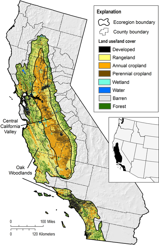
Figure 1. Study region in California including the Central California Valley and Central California Foothills and Coastal Mountains EPA Level III ecoregions [23], associated counties (outlined in light black) included in the study area, and 1992 land use and land cover.
Download figure:
Standard image High-resolution image2.2. State variables
We used the 1992 National Land Cover Dataset (NLCD92) [27] to define our initial LULC state class categories. The 20 original NLCD92 LULC categories were aggregated into primary LULC categories as defined in table 1. To identify areas with high levels of protection, where future land use activities would be limited or prohibited, we used data from the US Geological Survey's Protected Area Database [28] to classify rangeland and forest into protected versus unprotected. The LULC state of each cell was then based on a nearest neighbor resampling of the NLCD92 (30 m) and protected areas maps to 1 km2. A total of 1104 unique state class combinations were available, as a result of combining 12 LULC classes from table 1 with the two ecoregions and 46 counties. For the perennial cropland class we tracked both age and time-since transition (TST).
Table 1. State classes and the corresponding classes from the 30 m National Land Cover Dataset. Descriptions closely follow those outlined in Anderson et al [33] and Sleeter et al [25].
| State class | Area (km2) | % of study region | NLCD classes | Description |
|---|---|---|---|---|
| Rangeland | 52 866 | 36.1% | Grasslands/herbaceous shrublands | Land where potential natural vegetation is predominantly grasses, grass-like plants, forbs, shrubs, or brush and where natural herbivory was an important influence in its pre-civilization state. The vegetated cover must comprise at least 10% of the area. |
| Rangeland (protected) | 11 217 | 7.7% | Grasslands/herbaceous shrublands | Same as the rangeland class but set aside for permanent exclusion from conversion to an alternate land-use or land-cover state. |
| Annual cropland | 33 127 | 22.6% | Pasture/hay row crops small grains, fallow | Non-woody cropland or pastureland in either a vegetated or non-vegetated state used for the production of food and fiber. |
| Perennial cropland | 10 550 | 7.2% | Orchards/vineyards/other | Woody cropland persisting over multiple growing seasons used for the production of food, drink, and fiber, that does not get destroyed or removed during harvest. |
| Forest | 16 761 | 11.4% | Deciduous forest, evergreen forest, mixed forest | Tree-covered land where the tree-cover density is greater than 10%. |
| Forest (protected) | 7071 | 4.8% | Deciduous forest, evergreen forest, mixed forest | Same as the Forest class but set aside for permanent exclusion from conversion to an alternate land-use or land-cover state. |
| Developed | 9500 | 6.5% | Low intensity residential, high intensity residential, commercial/industrial/transportation, urban recreational grasses | Areas of intensive use with much of the land covered with structures (e.g., high density residential, commercial, industrial, transportation, mining, confined livestock operations), or less intensive uses where the land cover matrix includes both vegetation and structures (e.g., low density residential, recreational facilities, cemeteries, etc), including any land functionally attached to the urban or built-up activity or in a non-native vegetation state for human recreation. |
| Barren | 2642 | 1.8% | Bare rock/sand/clay | Land comprised of natural occurrences of soils, sand, or rocks where less than 10% of the area is vegetated. |
| Water | 1897 | 1.3% | Open water | Areas persistently covered with water, such as streams, canals, lakes, reservoirs, bays, or oceans. |
| Wetland | 719 | 0.5% | Woody wetlands, emergent herbaceous wetlands | Lands where water saturation is the determining factor in soil characteristics, vegetation types, and animal communities. Wetlands are comprised of water as well as vegetation. |
2.3. Model process overview
LUCAS simulates transitions between LULC state classes in annual timesteps. For this model we defined 6 transition types and 332 transition pathways (table 2). The processes represented by these pathways include changes between agricultural classes, agricultural expansion, agricultural contraction, orchard removal, urbanization, and protection of rangeland and forest. Within a given timestep, the order at which transitions occur is random for each Monte Carlo simulation.
Table 2. The set of all possible state class transition pathways developed for the model, organized by transition type, number of pathways, spatial stratification and the 'from' and 'to' LULC state class. The (All) value means that the transition pathways is applied to both the Central Valley and Oak Woodlands ecoregions; the (N/A) value represent a transition pathway not applicable at the given spatial stratification level.
|
2.4. Model parameterization
2.4.1. Transition targets
State class transition targets were used to model agricultural expansion, agricultural contraction, urbanization, land protection, and conversions from annual to perennial cropland. Transition targets for the agricultural expansion, agricultural contraction, and urbanization transition types were based on a time series derived from the California Farmland Mapping and Monitoring Project (FMMP), which provides land-use transition amounts for each of the 46 counties in the study area on a biannual basis for the historical 1992–2012 period (figure S1) [34, 35]. The FMMP data was directly used in the model for the 1992–2012 period. For the projected period (2012–2062) we randomly selected one of the FMMP historical years (and its corresponding change rates) for each timestep in each Monte Carlo. By randomly sampling one of the historical years we preserve the covariance of change rates between counties, as opposed to sampling each county independently.
There were no data available documenting the historical rate of change between annual and perennial cropland in California. Agricultural statistics indicate a trend towards increasing perennial and decreasing annual cropland over the last half of the 20th century [36], however, statistical surveys alone do not indicate the source of these trends, specifically the rate of individual class conversions. Within the model we assumed changes from annual cropland to perennial cropland occur at an average rate of 100 km2 yr−2 (standard deviation of 50 km2) from which we sample across every timestep and Monte Carlo simulation.
For the protection transition pathway, a map of areas protected between 1992 and 2011 was created and used to constrain the spatial location of rangeland and forest protection over the first 18 years of the simulation [28, 38–40]. For the future projections, a map of critical and priority areas for protection [41] was used to constrain the spatial location of new protected areas. Additionally, historical data on forest and rangeland protection were analyzed to produce a patch size class distribution of protected areas (table S1) to guide patch size of newly protected lands over the model period (2012–2062).
2.4.2. Transition probabilities
For the perennial cropland state class we tracked the age and TST for every cell to project the amount of orchard removal as well as transitions from perennial to annual cropland. No data exists on the age structure of perennial croplands in California, therefore age was initialized randomly for each cell using a uniform distribution between ages 1 and 45. In California, orchards are removed and/or replanted at an average age of 25 years, a decrease from ∼35 year old maturity in the 1980s [37]. As a result, the following parameters for orchard removal were established: (1) the minimum age of an orchard is 20, and (2) for each timestep and Monte Carlo simulation, the annual transition probability is sampled from a uniform distribution corresponding to a cumulative transition probability of 0.95 for ages 20 and 45 resulting in transition probabilities of 0.0228 and 0.0950, respectively. We assume orchard removal is followed immediately by replanting resulting in the state class remaining unchanged but with the age reset to zero. For the perennial to annual cropland pathways, we set a transition probability of 0.05 for all cells classified as perennial cropland and with a TST for orchard removal of 1 year. The effect of these parameters results in a 5% probability of orchards converting to annual cropland within 1 year of an orchard being removed. Lastly, we prohibit perennial cropland from transitioning to rangeland (agricultural contraction) or to annual cropland (agricultural change) until they are at least 20 years old.
2.4.3. Spatial multipliers
Spatial multipliers were used to constrain the location of allowable land-use change in two ways. First, we defined spatial adjacency rules for the agricultural change, expansion, contraction, and urbanization pathways. The probability of a cell experiencing any one of those transitions was calculated as a linear function of the proportion of the eight neighboring cells classified as the 'to class'. For example, the probability of a cell converting into developed (urbanization) was calculated based on the number of adjacent cells already classified as developed; the higher the number of adjacent cells classified as developed, the higher the calculated probability. If a cell has no neighbors classified in the 'to class' then the transition probability was set to zero.
In addition to the adjacency multipliers, spatial multipliers were used to constrain transitions on protected and managed lands [29, 30]. Spatial multipliers allow or constrain state class transitions and can be implemented on specific pathways. We set the probability of conversion for the agricultural expansion and urbanization pathways to zero for federal lands, including military installations and tribal lands [31], and protected areas where there was a management plan in place prohibiting anthropogenic land use [28]. In addition, we set the transition probability for urbanization to zero for agriculture lands currently enrolled in the Williamson Act, a conservation program within the State of California which provides economic incentives to agricultural land holders to maintain an agricultural land use [32].
2.5. Water use
In addition to tracking state class variables, the model was parameterized to track water use by county and state class type. To calculate average county applied water use for the annual and perennial cropland classes we: (1) determined the area of each crop type by county from the USDA Cropland Data Layer (CDL) [42]; (2) 'crosswalked' the CDL cropland types to the cropland categories associated with the California Department of Water Resources Agricultural Land & Water Use 1998–2010 dataset (CDWR) [43] (table S2); (3) collapsed the CDWR data into annual and perennial cropland classes and assigned an area-weighted average applied water use value for each combination of county and state class type (table S3). For the developed class, applied water use was derived from a national dataset of water use by various sectors [1].
Applied water use for the developed state class was calculated as follows:
where DevAWCTY1...n is developed state class (Dev) average applied water (AW) use for each county (CTY1...n), 'public supply-freshwater' (i.e. public supplied total freshwater withdrawals in kl yr−1) and 'industrial self-supplied' (i.e. industrial self-supplied total freshwater withdrawals in kl yr−1) are categories tracked within the CDWR data corresponding to urban and suburban, commercial, and industrial sectors, and Developed corresponds to the total developed area in each county based on the NLCD 2011 [46] developed state class (section 2.2, table 1).
2.6. Simulation experiments
The analysis described in this paper is the result of a single 'BAU' scenario. The BAU scenario was run over 70 timesteps (1992–2062); the first 20 years refer to the baseline historical conditions represented in the years 1992 through 2012. Projections were developed from 2012 through 2062. We ran 40 Monte Carlo simulations of the BAU scenario to reflect the variability in historical change rates and uncertainties associated with various model parameters.
2.7. Model validation
A pixel-level validation of the model used for this analysis was not possible due to the lack of a reference condition time series. The NLCD92 map used to establish initial conditions within the model represents a single date product, not directly comparable to later versions of NLCD due to changes in mapping methodology and classification scheme [27, 44–46]. However, we could validate that the internal calculations of the model functioned as expected by comparing the input transition demand to model simulation output. Additionally, we compared our simulated results over the baseline period with regional-scale data describing trends in land-use classes, providing important insight into the robustness of the modeling framework.
Structurally, the model consistently produces the expected outcome by matching the input transition target amounts. Figure S1 shows a comparison of the transition targets used to derive the BAU projections with the model simulations over the same temporal period (1992–2012). Mean model estimates are consistent with the transition targets; variability around the modeled mean results from the underlying sampling algorithm.
We compared our estimates of cropland (total, annual, and perennial) with statistical estimates from the National Agricultural Statistical Service (NASS) for the period 1992–2009 (figure S2) [36]. NASS estimated a net decline of 3.0% in harvested area, with a 13.6% decline in field crops and a 28.6% increase in fruit and nut crops. For comparison, LUCAS model simulations estimate a 2.4% decline in total agricultural land use, with a 10.2% decline in annual crops and a 22.0% increase in perennial crops. A true comparison is complicated due to definitional differences between crop categories, however, the overall modeled trends in agricultural land use are consistent with the broad trends identified in statistical estimates.
Additional comparisons were made for the rangeland and developed classes. For developed area we compared model estimates to the total estimated change from the FMMP data. FMMP projected an increase of 3152 km2 between 1990 and 2010 while our model estimated a net increase of 3328 km2 between 1992 and 2010. Rangelands were more difficult to compare since the definition of what lands are included in the category often vary. Furthermore, comparison using satellite data are problematic due to the change in mapping method between NLCD92 and versions from 2001 forward. For this reason we compared changes in rangeland (herbaceous grassland and shrub/scrub classes from NLCD) between 2001 [27] and 2011 [46] with our modeled estimates. NLCD estimated a net decline of −0.6% and the model produced an estimated net decline of −1.2%.
3. Results
Between 2012 and 2062 in the BAU scenario, developed land cover was projected to increase 62.9% from an average 12 978 km2 to an average 21 141 km2 (figures 2(a) and (b)). Annual cropland was projected to decline an average 30.3% (8822 km2). Conversion of annual cropland into perennial cropland and encroachment of perennial crops into rangeland resulted in perennial cropland increasing 39.1% (5192 km2). Overall, anthropogenic land uses increased over 8.2% (4533 km2) from 2012 levels at the expense of rangelands while total cropland area declined 8.6%. Continued additions of protected rangeland at the historical rate did not abate continued losses through mid-century. Rangelands continued to decline (−7.3%) despite the addition of 3211 km2 of protected rangeland in the BAU scenario.
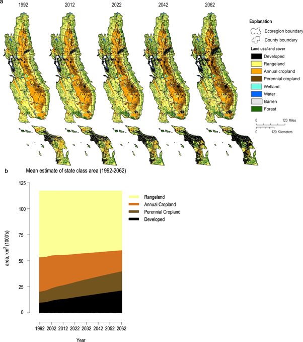
Figure 2. (a) Projected land-use and land-cover (LULC) change for the historical period (1992–2012) and the projected period (2012–2062) in California's Central Valley and Oak Woodlands regions under a business-as-usual (BAU) scenario. The 2012 and 2062 LULC maps represent one out of 40 possible Monte Carlo iterations modeled for each time step. See table 1 for a full explanation of the LULC classification scheme. (b) Trends in mean LULC change over the historical and projected period by LULC class.
Download figure:
Standard image High-resolution imageHistorical land use transitions persisted into the future under the BAU scenario. Conversions into developed land uses came predominantly from rangelands in the Oak Woodlands ecoregion (figure 3(a)) and from annual and perennial cropland in the Central Valley (figure 3(b)). Conversions from annual cropland into perennial cropland had the highest annual average LULC transition rate in the Central Valley. Rangelands across the study area were also converted to agricultural uses, with large amounts of land fluctuating annually between rangeland and annual cropland as some areas are cultivated while others are idled [47, 48].

Figure 3. Average annual land-use and land-cover (LULC) change in square kilometers (km2) over the modeled period (2012–2062) for the (a) Oak Woodlands and (b) Central California Valley ecoregions as defined 'from' and 'to' LULC classes for transitions between annual cropland (A; orange), perennial cropland (P; brown), rangeland (R; yellow), and developed (D; gray) classes (e.g. A–D represents transitions from annual crops to developed land with box fill color representing the 'to' LULC class). Boxes indicate the 'to' LULC class and the 25%–75% range and median (line), box fill color represents the 'to' class for the transition, while whiskers indicate the 5%–95% range and dots represent outlier county values.
Download figure:
Standard image High-resolution imageBy 2062, water use was projected to increase by 1.8 billion cubic meters (Bm3; +4.1%) over current use estimates (figure 4). Within the developed sector, water use demand was projected to increase 4.6 Bm3 (+59.1%) from an average 7.9 Bm3 (range of 7.8–7.9 Bm3) in 2012 to an average 12.5 Bm3 (range of 12.0–13.0 Bm3) in 2062. This represents a 9.4% increase (from 17.8% to 27.3%) in the develop sectors proportion of total regional water use. For the annual cropland sector, water use was projected to decline nearly 30.2% or an estimated 7.3 Bm3 (range of −6.8 to −7.9 Bm3) while perennial cropland water use was projected to increase by 4.5 Bm3 (range of 3.9–5.1 Bm3) or 37.5%. Combined, total cropland water use was projected to decline 2.8 Bm3 from an average 36.2 Bm3 in 2012 to 33.4 Bm3 in 2062 representing a 7.8% decrease in agriculture water use (figure 4).

Figure 4. Projected net change in water use demand from 2012 to 2062 for agriculture and developed (municipal and industrial) water use expressed in millions of cubic meters (106 m3), including average (bar) and maximum and minimum value ranges across 40 Monte Carlo simulations.
Download figure:
Standard image High-resolution imageAt the county scale, annual cropland losses to perennial cropland and development drove net increases in water demand. Large gains in developed land use led to net increases in water use in Alameda, Los Angeles, Orange, Riverside, Sacramento, San Diego, and Ventura counties, where urbanization of rangelands was projected to occur and large population centers already exist (figure 5(a)). San Diego County exhibited the highest net increase in projected water use, almost entirely attributed to the development of rangelands (see also figure 2). In 82% of counties, net demand for water increased (figure 5(b)). Net declines in water demand were projected where losses of annual cropland exceeded gains of perennial cropland and new developed land (e.g. Kern and Kings Counties).

Figure. 5. Average change in water use demand between 2012 and 2062 in cubic meters for each county in the study region by (a) land use category and (b) net change in overall water use. Boxes indicate the mean (+), median (line), and 25%–75% range, while whiskers indicate the 5%–95% range and dots represent outlier county values.
Download figure:
Standard image High-resolution image
4. Discussion and conclusions
The results presented in this research highlight several key issues likely facing California water users and managers in the future, if current trends persist. In 38 of 46 counties our model results show a net increase in overall projected water use. Our results indicate that currently mandated 25% municipal water use restrictions would need to be maintained through 2062 for future water demand to remain at or below 2012 demand. Water use in 2012 was already proven unsustainable given the ongoing multi-year drought, which lead to mandated municipal use restrictions in 2015. Reaching current 2015 use levels in 2062 would require some combination of increased use efficiencies across sectors and/or new supplies [51]. It has been estimated that nearly one-third of municipal water use in California could be saved if all existing technologies were implemented [52]. Current data indicate perennial cropland expansion continues, driven by increases in the total value of almonds from $4.8 billion in 2012 to $6.4 billion in 2013, followed by grapes at $5.6 billion [53]. California's continued population growth projections will undoubtedly lead to new developed land use as well [18]. It is important to note that any new demand for water will also require additional energy for transport and delivery. Storage and redistribution of California's water already consumes nearly 20% of the state's electricity and 30% of its natural gas [54].
The projected trend in declining agricultural water use reflects the observed historical trend of regionally intensive urbanization of farmland, as well as the trend towards more high risk and high value perennial crops [36]. Almonds are the fourth most water intensive crop in California and the state's largest agricultural export by value, second only to hay in total acreage planted [50]. As a result, in only 16 of 46 counties was historical perennial cropland water use lower than water use for annual crops. Improvements or changes in water use efficiency and crop yields were not considered in this study and reflect a key uncertainty when projecting future water use demand. Since 1992, the water use efficiency of orchards and vineyards has increased 28% and 33% respectively [49] while crop yields have also increased [56]. The BAU scenario assumes no additional improvements in efficiency due to technological advancements.
There was considerable uncertainty associated with transitions within the agricultural sector, specifically the conversion between annual and perennial cropland categories. Additionally, little is known about the current age structure of orchards in California. As orchards reach maturity and decline in production, land owners must decide whether to replant perennial crops or switch to a different land use. Improved mapping techniques using remotely sensed data should be evaluated as they mature to better inform some of the important data gaps associated with LULC change in California.
Future climate variability can also have positive and/or negative impacts on water use, in terms of reduced water availability due to decreased precipitation and higher evaporative loss due to temperature increases, but may also result in increased production due to warming and the effect of CO2 fertilization. Furthermore, climate can have positive and/or negative feedbacks on future land use (e.g. less precipitation, less water availability, more applied water use per crop, lower potential for agricultural expansion). While the 1992–2012 FMMP land change data do include two drought episodes, including the 2007 onset of the current, extreme drought, land use decisions based on long-term water shortages were not fully captured. These are important considerations which were outside the scope of this study, yet need to be recognized as important limitations and uncertainties which should be incorporated into future work.
Future changes in land use were based on a 20 year historical record which spans a wide range of climatic and socioeconomic conditions. The projections derived from these data cover a wide range of future conditions, but do not represent all future possibilities. Additional work should be undertaken to develop alternative 'what-if' scenarios to explore how significant departures from historical conditions (extreme events) could impact regional water use demand. One such example would be if California entered into a prolonged long-term drought. Even short duration events (4–6 years) have shown to have strong feedbacks on land-use change dynamics [57].
Land-use projections provide a previously unseen view into potential water use futures. This information is essential for water management agencies and a broad array of stakeholders given the state's economic dependency on this already over-allocated resource [2]. Agriculture use values are often grossly underestimated by as much as 20%–30% [49, 55], as they are often not measured directly, but calculated based on crop acreage, crop coefficients, stage ratios, irrigation-system efficiency, and precipitation [1]. Estimates on public water use are generally more accurate and based primarily on site-specific information [1]. Considering probable underestimation, increasing demand for water in coming decades is likely greater than our projections indicate. This may eventually force a reconciling of human and ecosystem water needs, particularly in the face of projected climate-driven declining supplies.
Acknowledgments
This research was supported by the US Geological Survey's Climate and Land Use Research and Development Program, the USGS Land Change Science Program, and funding from The Nature Conservancy. We are grateful for the detailed and thoughtful internal peer review provided by Dr Claudia Faunt and our anonymous peer reviewers.
Model and data access
All modeling for this study was done using the ST-SIM software application which can be downloaded free of charge from APEX Resource Management Solutions (http://apexrms.com). All model parameters are available as (1) a Microsoft Excel file and (2) a database containing all model inputs and outputs (http://geography.wr.usgs.gov/LUCC/).