

Abstract
The urban heat island effect is a phenomenon observed worldwide, i.e. evening and nocturnal temperatures in cities are usually several degrees higher than in the surrounding countryside. In contrast, cities are sometimes found to be cooler than their rural surroundings in the morning and early afternoon. Here, a general physical explanation for this so-called daytime urban cool island (UCI) effect is presented and validated for the cloud-free days in the BUBBLE campaign in Basel, Switzerland. Simulations with a widely evaluated conceptual atmospheric boundary-layer model coupled to a land-surface model, reveal that the UCI can form due to differences between the early morning mixed-layer depth over the city (deeper) and over the countryside (shallower). The magnitude of the UCI is estimated for various types of urban morphology, categorized by their respective local climate zones.
Export citation and abstract BibTeX RIS

Content from this work may be used under the terms of the Creative Commons Attribution 3.0 licence. Any further distribution of this work must maintain attribution to the author(s) and the title of the work, journal citation and DOI.
1. Introduction
Currently, cities are confronted with major challenges regarding ongoing urbanization and the impacts of climate change [1]. About 52% of the 7.3 billion people reside in urban areas, which is foreseen to increase to 67% in 2050 [2]. In addition, the globally averaged near-surface air temperature is projected to raise further, in conjunction with a projected increase in the abundance of heat waves in many parts of the world [3, 4]. Both developments underline the need to understand the environmental physics of the urban environment since this directly governs health, well-being and labor productivity of urban dwellers through thermal comfort, air quality and the alteration of the flow around buildings.
The urban land use strongly influences the energy and water balance and impacts city weather and climate. The urban heat island effect (UHI) is the most profound meteorological contrast between cities and the countryside, i.e. the urban temperature exceeds the rural temperature, particularly in the evening and at night; in some cases more than 8 K [5–7]. The UHI is driven by a variety of processes. The most important of which are the excess heat stored in the city during the day, which is subsequently released during the night [8] and anthropogenic heat release.
The UHI has been the focus in many studies; while a significant number of these studies document that cities often remain cooler than the countryside from the early morning until the early afternoon during fair weather and low wind speed conditions. This so-called urban cool island (UCI) may amount to 1–2 K [9–14]. The UCI has been both observed and forecasted using atmospheric models [15, 16], earlier studies qualitatively suggest that the UCI may originate from shadow effects in the urban canyon [7, 8], the daytime energy storage in the urban fabric [13], the attenuation of net radiation due to aerosols [12], or the difference in land cover and the available soil moisture altering the surface energy balance [17, 18]. The current study explores an extended and more general physical explanation for the UCI that is rooted in atmospheric boundary-layer (ABL) dynamics.
The ABL is defined as the turbulent layer of the atmosphere closest to the Earth's surface [19]. At night, the rural ABL cools and can be relatively shallow (∼ 100 m, [20, 21]). On the other hand, the urban nocturnal ABL remains substantially deeper (∼400 m) [8, 21] because it remains supplied with heat stored in buildings during the day, the storage or ground heat flux. Here, we hypothesise that the difference between the thin rural ABL and the thick urban ABL causes a difference in heating rates between the urban and the rural environment in the early morning. As such, we expect that the countryside will warm up faster than the urban environment since the layer overlying the countryside is thinner and has a lower volume than the urban ABL.
The hypothesis will be evaluated using prognostic equations for the ABL height and potential temperature. This conceptual ABL model is initialized and evaluated with observations during the BUBBLE campaign in Basel, Switzerland [13, 22], where the UCI effect was observed during the intensive observation period (IOP) in the summer of 2002. Furthermore, the sensitivity of the modelled UCI will be tested for a variety of ABL and urban surface properties.
2. Methodology
2.1. Model formulation
Our hypothesis is based on the daytime ABL evolution and consequently a conceptual mixed-layer model [23] is appropriate to study the UCI. This mixed-layer model has been widely evaluated [24–26], and has been successfully applied to study the impact of aerosols [27], land–atmosphere coupling [28, 29], clouds [30], carbon dioxide [31] and urban areas [32] on the ABL.
The mixed-layer model is a bulk model for the boundary layer and consists of a uniform virtual potential temperature ( ) and specific humidity (
 ) below a sharp potential temperature (
 ) and specific humidity inversion (
 ) at the ABL top (h), and a linear increase (decrease) in the potential temperature (specific humidity) in the free atmosphere aloft (see figure 1).

Figure 1. Schematic overview of the urban and rural ABL around sunrise. The potential temperature profiles display the schematic representation of the urban and rural ABL. The dashed line denotes the height of the rural (green) and urban (red) boundary layer.
Download figure:
Standard image High-resolution imageThe set of mixed-layer equations is described by:


This numerical bulk model is applied to the urban and the rural ABL and advection is neglected. In the set of equations, b is the fraction of energy added by entrainment of warm free tropospheric air at the top of the ABL and amounts to −0.2, which is a ratio widely used to simulate the convective ABL in low wind speed cases [19, 33]. Furthermore, the free tropospheric lapse rate is denoted by  and subsidence velocity by wL.
In order to represent the interactive processes between the land surface and the ABL, the surface fluxes for heat ( ) and moisture (
 ) are calculated using a coupled land-surface parameterization valid for clear-sky conditions. The coupling of a land-surface parameterization gives realistic diurnal variations in the surface fluxes and allows for studying the sensitivity to urban surface properties. The evolution of the surface temperature is calculated as follows [34]:

Here, c is the heat capacity per unit area and  is the surface skin temperature.
  is the net radiation. Special care is taken to the storage or ground heat flux (
 ) as this is one of the driving factors for the UHI and thus the higher urban ABL during the night. The storage heat flux is calculated following the objective hysteresis model [35], and H and LvE are the sensible and latent heat flux calculated using the Businger–Dyer relationships [36]. More detail is given in the supplementary material.
In order to evaluate model results with observations at pedestrian level, we estimate the surface-layer air temperature from the ABL temperature using [37]:

Here, rah is the aerodynamic resistance, ρ the air density and Cp the specific heat capacity of air. We use a rural reference height z = 2 m, while in the urban environment this is more complex. Therefore, a two-step approach is used to evaluate the model performance in an urban area: first we evaluate the temperature above the roughness sublayer, followed by the evaluation of the air temperature in the urban canyon (see section 3.1).
2.2. Observations
The BUBBLE campaign is one of the rare datasets where boundary-layer observations are combined with surface observations and turbulent fluxes for both urban and rural sites and we are limited to this data from Basel, Switzerland [13]. In this study we selected the fair-weather days during the IOP in the BUBBLE campaign (one month during the summer of 2002), as these are conditions that are favourable for UCI formation [11]. During this IOP there were 8 fair-weather days, of which one is described in detail here, the other cases can be found in the supplementary material.
Table 1 shows the initial conditions used in the mixed-layer equations for 26 June, 2002 (other cases described in table S2). The simulation is started at 5:00 local time (LT) with the observed ABL-UHI of 1 °C and the observed urban and rural boundary-layer depths of 400 and 100 m, respectively. The urban simulations are initialized and validated with data from site Basel-Spalenring (47.555 N; 7.576 E). The urban ABL height is estimated to be the aerosol mixed-layer height obtained from a Lidar situated at this site, where we assume an uncertainty of about 200 m [38]. The rural simulations are initialized and validated with data from site Grenzach (47.537 N; 7.675 E). The rural ABL height is estimated from the vertical velocity of a doppler sodar system at this site. To this end we assumed the standard deviation of the vertical velocity was larger than  in the ABL. The sensitivity to the initial ABL profiles is documented in section 3.3
Table 1. List of the default input variables into the mixed-layer equations as observed during 26 June, 2002 in Basel, Switzerland.
| Variable | Rural | Urban | |
|---|---|---|---|
| Initial mixed-layer potential temperature |

|
287 K | 288 K |
| Initial mixed-layer temperature inversion |

|
5 K | 4 K |
| Potential temperature lapse rate |

|
0.007 
|
0.007 
|
| Initial mixed-layer humidity |

|
8.7 g kg−1 | 9.1 g kg−1 |
| Initial mixed-layer humidity inversion |

|
−0.1 g kg−1 | −0.1 g kg−1 |
| Humidity lapse rate |

|
−0.001 g kg−1m−1 | −0.001 g kg−1m−1 |
| Initial boundary-layer height | h0 | 100 m | 400 m |
| Subsidence velocity | wL | −0.00324 
|
−0.00324 
|
Subsidence is derived from the European Centre for Medium-Range Weather Forecasts reanalysis vertical velocity above the ABL, averaged over the entire day [39].
2.3. Experimental set-up
The following numerical experiments are used to test whether the UCI is formed due to the higher early-morning urban ABL compared to the rural ABL height:
Experiment 1. This is the default experiment with an urban and rural mixed layer initialized with values from table 1. The parameters used in the land-surface parameterization are described in table S1.
Experiment 2. This experiment determines the sensitivity of the UCI to the thermodynamic state of the ABL and surface conditions. Here,  h0,
h0,  and the maximum sensible heat flux (
 ) are varied.
  between 1 °C and 8 °C. h0 between 30 and 500 m (rural), and 50 and 1000 m (urban).
  between 0.0001 and 0.01
 between 80 and 290 (rural), 230 and 470
  (urban).
Experiment 3. This experiment determines the sensitivity of the UCI for different urban landuse types. Here, the surface emissivity, albedo, roughness length, building height, anthropogenic heat, vegetation fraction, and initial boundary-layer height (table 2) are varied for each of the 10 local climate zones (LCZs) described in section 2.4.
Table 2.
A list of the local climate zones and their in- and output properties: surface emissivity  albedo α, roughness length z0, building height zh, vegetation fraction
  anthropogenic heat
  initial boundary-layer height h0, sensible heat fraction of the net radiation
  Bowen ratio
  maximum heating rate
  and maximum boundary-layer growth rate
| LCZ |

|
α | z0 | zh |

|
AHmax | h0 |

|

|

|

|
|---|---|---|---|---|---|---|---|---|---|---|---|
| (-) | (-) | (m) | (m) | (-) | (
|
(m) | (-) | (-) |

|
 ) ) |
|
| (1) Compact high-rise | 0.91 | 0.13 | 6.75 | 45 | 0.05 | 50 | 500 | 0.48 | 12.0 | 1.61 | 204 |
| (2) Compact mid-rise | 0.91 | 0.18 | 1.5 | 12 | 0.10 | 17.5 | 480 | 0.46 | 6.0 | 1.50 | 196 |
| (3) Compact low-rise | 0.91 | 0.15 | 0.4 | 5 | 0.15 | 15 | 459 | 0.46 | 4.0 | 1.58 | 207 |
| (4) Open high-rise | 0.91 | 0.13 | 5.25 | 40 | 0.35 | 15 | 375 | 0.30 | 1.7 | 1.41 | 174 |
| (5) Open mid-rise | 0.91 | 0.13 | 1.25 | 15 | 0.30 | 7.5 | 396 | 0.34 | 2.0 | 1.47 | 186 |
| (6) Open low-rise | 0.91 | 0.13 | 0.5 | 5 | 0.40 | 5 | 354 | 0.33 | 1.5 | 1.54 | 192 |
| (7) Lightweight low-rise | 0.28 | 0.15 | 0.2 | 3 | 0.15 | 15 | 459 | 0.56 | 4.0 | 1.76 | 235 |
| (8) Large low-rise | 0.91 | 0.18 | 0.55 | 7 | 0.15 | 20 | 459 | 0.40 | 4.0 | 1.41 | 182 |
| (9) Sparsely built | 0.91 | 0.13 | 0.35 | 5 | 0.70 | 2.5 | 227 | 0.27 | 0.9 | 1.73 | 206 |
| (10) Heavy industry | 0.91 | 0.10 | 1.1 | 8.5 | 0.45 | 150 | 232 | 0.32 | 1.3 | 2.66 | 290 |
| Rural | 0.99 | 0.2 | 0.1 | — | 1.00 | — | 100 | 0.25 | 0.6 | 2.71 | 265 |
2.4. Local climate zones
In experiment 3 the sensitivity of the UCI formation is tested for different urban landuse types. These properties will alter the surface fluxes, leading to differences in the ABL growth, temperature and UCI. In addition, h0 will vary for different urban types. A classification of urban morphology is provided by LCZ [40, 41]. This classification system is applicable worldwide and designed to couple typical land-use characteristics, such as surface type, structure and anthropogenic activity, to the local thermal climate. Each LCZ has characteristic values for the urban surface properties, such as albedo, emissivity, aspect ratio, impervious, pervious and building surface fractions and anthropogenic heat production (see table 2).
The anthropogenic heat is added to the sensible heat flux using a sinusoidal function with two peaks at 8:00 in the morning and 16:00 in the afternoon LT during the rush-hours, similar to previous research [42]. The added heat is increasing the urban sensible heat flux especially in the morning and potentially decreases the UCI intensity. Urban areas with added vegetation are expected to have the opposite effect and decrease the sensible heat flux during the day and enhance the UCI.
The surface characteristics are based on previous studies [40, 41], which have shown that more urbanised areas have a larger storage flux capacity, causing the ABL to remain higher. Sparsely built areas, on the other hand, do not store as much energy and the ABL can become stable as in the rural area. Based on this assessment we have tried to estimate a 'characteristic' h0 for each LCZ, using only the vegetation fraction ( ) for simplicity. This results in the following linear assumption for the initial ABL height for each LCZ:

Here, hurban is the initial boundary-layer height for each urban type or LCZ, hrural the rural ABL height and href is a reference height. For calibration, we use the reference day (26 June, 2002, section 2.2) from the BUBBLE data set (

 and consequently
  m). Equation (7) indicates that hurban increases for cities with less vegetation as one would anticipate.
3. Results
3.1. Model validation
From all 8 fair weather days during the BUBBLE IOP (section 2.2), 26 June, 2002 is described in more detail below. Results for the other cases are given in the supplementary material.
At the observational site, temperature, observations at 3 and 33 m above the surface are available. First, we use equation (6) to calculate  i.e. at 2.64 times the building height which is assumed to be above the roughness sublayer height. Subsequently, we evaluate
  against observations. Figure 2(a) shows that the modelled 33 m potential temperature compares very well with the observed temperature measurements at 33 m (root mean squared error (RMSE) = 0.71 K, MEAE [median absolute error] = 0.65 K), and thus we may conclude that the model can successfully simulate
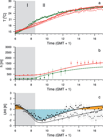
Figure 2. Diurnal evolution of the modelled (lines) and observed (markers) air temperature (a), boundary-layer height (b) and the urban heat island (c) in the urban (red) environment at 33 m (dotted lines and stars), at 3 m (solid lines and dots) and rural (green dashed lines and squares) environment. The measurements are for 26 June, 2002 at the urban measurement site Basel-Spalenring and the rural site Grenzach [13].'I' indicates the heating phase and 'II' the growing and heating phase (section 3.2).
Download figure:
Standard image High-resolution imageIn the next step, we estimate the air temperature in the canyon. Therefore, the canyon sensible heat flux is estimated using an empirical method [22] that accounts for the divergence of the sensible heat flux in the roughness sublayer. The estimated canyon heat flux is then used to estimate the temperature from 33 m down into the urban canyon at 3 m. Consequently, the modelled canyon temperature in figure 2(a) shows a remarkable resemblance to the observed 3 m canyon temperature (RMSE = 0.56 K, MEAE = 0.42 K). Finally, the rural 2 m temperature is also very close to the observations (RMSE = 0.49 K, MEAE = 0.26 K).
3.2. UCI formation
The model is initialized at sunrise with an urban ABL that is deeper (400 m) than the ABL over the rural area (100 m) following the observations (figure 1). Note that these initial ABL heights are almost the same as found for London [21]. Figure 2 shows the modelled diurnal evolution of the convective ABL height, the air temperature and the UHI.
In the first 3.5 h after sunrise we find a heating phase with increasing temperatures over both the urban and rural area. During this phase the ABL is only heated by the input of the surface heat flux, while the ABL growth is marginal (figure 2(b)). Although the urban surface heat flux is larger (∼110  ) than the rural surface flux (∼50
  ), the urban heating rate is lower than the rural heating rate (maximum of 1.49 versus 2.71
  ) because the volume of air in the urban ABL that needs to be heated is much larger than the volume of air in the rural ABL (see equation (1)). This finding corresponds to the earlier observations of a smaller heating rate in the urban environment compared to the rural environment [8, 43, 44].
The larger heating rate in the rural environment causes the rural temperature to become higher than the urban temperature in the morning some two hours after sunrise. This causes the initial UHI (of 1 K) to shift to an UCI effect, with a maximum value of ∼2 K (figure 2(c)) approximately 4 h after sunrise.
In the second growing and heating phase, both the urban and rural ABL start to grow and warm from around 8:30 h due to the entrainment (mixing in of warm air from free tropospheric air) into the ABL (see equation (3)). In this phase, the urban temperature increases more rapidly than the rural temperature due to the higher surface sensible heat flux of the city (maximum of ∼330 versus ∼180  ) (figure S1). Ultimately, the urban temperature exceeds the rural temperature around 13:30 LT. This effect is also confirmed by the BUBBLE observations, which emphasizes the robustness of the proposed UCI mechanism.
Alternative explanations for the UCI such as shading, uptake of energy and the limited availability of soil moisture in the rural surroundings all stem from an alteration in the energy balance [7, 8, 17, 18]. This would, however, likely require the sensible heat flux of the rural environment to be higher than that of the urban environment. This is not shown to be the case here (figure S1(a)). The sensitivity of the UCI to the sensible heat flux will be further explored in section 3.3.
Note that all the available days during the BUBBLE IOP with a potential for UCI formation show approximately similar results as the case presented here (see figures S2 and S3).
3.3. Sensitivity to the thermodynamic state of the boundary layer
The simulations suggest that the UCI basically forms due to the difference in the ABL depths at sunrise and disappears in the afternoon due to the higher surface sensible heat flux of the city compared to the countryside. Therefore, experiment 2 explores the sensitivity of the UCI magnitude to the initial ABL depth over the two terrain types, as well as to the free atmospheric lapse rate, the initial temperature inversions at the ABL top and the sensible heat flux calculated by the land-surface parameterization (figure 3).
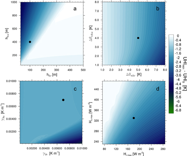
Figure 3. The sensitivity of the urban cool island to the initial boundary layer state and the maximum sensible heat flux. The maximum urban cool island (from the near-surface air temperature) subtracted by the initial urban heat island as a function of the initial rural (x-axis) and urban (y-axis) ABL heights h0 (a), temperature inversions  (b), free tropospheric lapse rate
  (c) and the maximum surface sensible heat flux
  (d). The black dot indicates the values in the default simulations.
Download figure:
Standard image High-resolution imageFigure 3 indicates that the difference in initial ABL height is the only factor to trigger the UCI (figure 3(a)). The UCI is only zero when the initial ABL height of the urban area is less than twice the initial ABL height over the rural area. For example, if the initial rural ABL height stays at 100 m, but the initial urban ABL is only 200 m instead of 400 m, the UCI is almost non-existent. In that case, the higher urban sensible heat flux heats up the urban ABL as fast as the rural ABL is heated up, giving the rural and urban area the same temperature in the morning.
The UCI magnitude is sensitive to the temperature inversion ( ) at the top of the rural ABL (figure 1), as a result of the shallower ABL in the growing phase (figure 3(b)). The UCI increases if
  is stronger, because it takes longer for the convection to break through the inversion layer and allowing the ABL to grow. This increases the duration of the heating phase in the rural environment, leading to a larger UCI (figure 3(b)). For example, increasing the
  by 1 K, the UCI increases to ∼2.5 K and lasts at least to 18:00 LT. On the other hand, decreasing the
  by 1 K causes the UCI magnitude to decrease to ∼1.5 K and only lasts until 11:30. Changes in the initial urban temperature inversion have a much smaller effect on the magnitude of the UCI.
Figure 3(c) shows the dependence of the UCI on the free tropospheric lapse rate. In the reference simulation for the selected BUBBLE day we use the same  =
=  in both the urban and rural environment. Note that the observed
  for the current day is in close agreement with values reported elsewhere of about 0.005–0.006
  [45, 46]. The figure shows that with an infinite residual layer (e.g.
  =
=  throughout the entire simulation, [47]) above the rural ABL, the formation of the UCI is not impacted (since the UCI does not vanish for a low
  ). On the other hand, an infinite urban residual layer amplifies the UCI because it allows for a rapid entrainment. This causes the ABL to grow more quickly and increases the area to be heated further, leading to a lower heating rate and a larger UCI.
Figure 3(d) shows the dependence of the UCI on the diurnal maximum of the sensible heat flux. When the urban sensible heat flux increases the urban temperature increases as well and the UCI decreases. However, if the sensible heat flux in the rural environment increases the rural heating rate becomes larger and the UCI as well.
3.4. Sensitivity to urban types
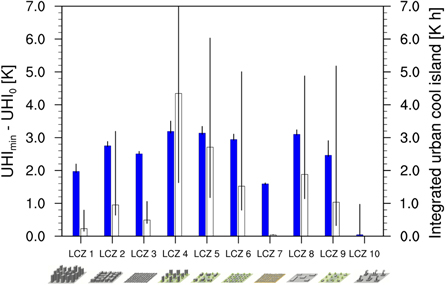
In experiment 3 we estimate the UCI in a similar manner as in experiment 1 for each LCZ, varying not only the surface properties but also the h0 and  This strategy provides a more general characterization of the UCI for real-world urban morphologies. Table 2 shows the fraction of sensible heat to net radiation, Bowen ratio and the resulting maximum heating rate and ABL growth rate for each LCZ. Figure 4 shows the maximum and integrated UCI for all 10 LCZs. The integrated UCI (UCIINT) is defined as
  for
for  and represents the 'dose' of the UCI during its presence. As such this is a better proxy for the day–time cooling potential than the maximum UCI magnitude alone.
Figure 4. The simulated urban cool island in different local climate zones. The maximum urban cool island (from the canyon temperature) subtracted by the initial urban heat island is indicated by the dark blue bars. The urban cool island dose, the integrated light blue area in figure 2(c) is displayed in the transparent bars. For each of the local climate zones specific initial values and surface characteristics are used (table 2),[41]. The error bars show the range of values with a varied urban ABL temperature inversion between 2 K and 6 K, default is 4 K.
Download figure:
Standard image High-resolution image
The magnitude of the modelled maximum UCI for each LCZ is substantial except for heavy industry (LCZ 10). For the other LCZs the maximum UCI does not have a very large range, from 1.6 K for LCZ 7 to 3.2 K for LCZ 4. In the case of heavy industry the high anthropogenic heat flux leads to a higher sensible heat flux in the early morning. In addition, the high vegetation fraction yields a lower ABL. The combination of these two effects causes a higher heating rate (∼2.66  ) in such urban areas resulting in a negligible UCI.
The zones with a relatively large areal vegetation fraction, but with a substantial h0 (LCZ 4-6 ) show a large UCIINT. This means that due to the lower sensible heat flux ( between 1 and 2) the UCI can last longer throughout the day. In zones with limited vegetation (e.g. LCZ 1-3) the heating rate in the urban area is still limited (∼1.5–1.6
  ) due to the deep urban ABL (∼460–500 m). However, the large sensible heat flux in these areas warm the ABL more during the heating and growing phase, limiting the duration of the UCI.
Figure 4 also shows that the maximum UCI is not very sensitive to  (figure 3(a)). However, the duration of the UCI is sensitive to this parameter. A smaller
  gives a larger UCIINT and vice versa. This means that with a small
  the ABL is able to grow more quickly, and the energy from the sensible heat flux has to be diluted over a deeper layer, resulting in a limited increase in the urban air temperature, and increasing the duration of the UCI.
4. Conclusions
Cities are generally known for the evening and nocturnal UHI effects. Surprisingly, cities have been reported to be cooler in the morning and early afternoon. Our experiments provide a general explanation for this UCI. The nocturnal heat release from the urban surface leads to a deeper ABL over the city than over the countryside at sunrise. This difference in ABL depth induces a higher early morning heating rate over the countryside than over the city. Consequently, the initial UHI at the end of the night progresses into an UCI. This UCI peaks about 4 h after sunrise and can last into the early afternoon. For a case with an initial boundary-layer UHI of 1 K and urban and rural ABL heights of 400 and 100 m, the UCI reaches up to 2 K.
The magnitude of the UCI and its duration strongly depend on the urban morphology. Anthropogenic heat increases the sensible heat flux in the urban area, especially during the morning and leads to a decrease in the UCI magnitude. A higher vegetation fraction has the opposite effect: a decrease in sensible heat flux and an increase in the UCI.
This research paves the way for new studies and could be extended to different cities. However, a limitation is the current lack of simultaneous measurements of the atmospheric boundary layer over urban and rural surfaces. In addition, the results of this study highlight the importance of including ABL dynamics in urban climate studies. Mesoscale atmospheric models can be used to elaborate this further. Different research perspectives also include the UCI implications for urban planning, health and air quality. The strong link between the UCI magnitude and the urban morphology indicates that the UCI can be employed as an efficient tool in urban planning and health.
Acknowledgments
This research was supported by NWO project CESAR as part of the program 'Sustainable accessibility to the Randstad' (grant 434_09_012). GJ Steeneveld and RJ Ronda acknowledge funding from NWO—EScience project 'Summer in the City' (grant 027.012.103). In addition, we would like to acknowledge funding from the WIMEK research fellowship for MW Rotach. Finally, we thank Jordi Vilà and Folmer Krikken for fruitful discussions.