Self-consistent dynamical field theory of kernel evolution in wide neural networks^*

A natural extension to the lazy NTK/NNGP limit that allows the study of feature learning is to calculate finite width corrections to the infinite-width limit. Finite width corrections to Bayesian inference in wide networks have been obtained with various perturbative [23–29] and self-consistent techniques [30–33]. In the GD based setting, leading order corrections to the NTK dynamics have been analyzed to study finite width effects [27, 34–36]. These methods give approximate corrections which are accurate provided the strength of feature learning is small. In very rich feature learning regimes, however, the leading order corrections can give incorrect predictions [37, 38].

Another approach to studying feature learning is to alter NN parameterization in gradient-based learning to allow significant feature evolution even at infinite-width, the mean field limit [21, 39]. Works on mean field NNs have yielded formal loss convergence results [40, 41] and shown equivalences of gradient flow dynamics to a partial differential equation (PDE) [42–44].

Our results are most closely related to a set of recent works which studied infinite-width NNs trained with GD using the TPs framework [22]. We show that our discrete time field theory at unit feature learning strength $\gamma_0 = 1$ recovers the stochastic process which was derived from TP. The stochastic process derived from TP has provided insights into practical issues in NN training such as hyper-parameter search [45]. Computing the exact infinite-width limit of GD has exponential time requirements [22], which we show can be circumvented with an alternating sampling procedure. A projected variant of GD training has provided an infinite-width theory that could be scaled to realistic datasets like CIFAR-10 [46]. Inspired by Chizat and Bach's work on mechanisms of lazy and rich training [17], our theory interpolates between lazy and rich behavior in the mean field limit for varying γ₀ and allows comparison of DMFT to perturbative analysis near small γ₀. Further, our derivation of a DMFT action allows the possibility of pursuing finite width effects.

Our theory is inspired by self-consistent DMFT from statistical physics [47–53]. This framework has been utilized in the theory of random recurrent networks [54–59], tensor PCA [60, 61], phase retrieval [62], and high-dimensional linear classifiers [63–66], but has yet to be developed for deep feature learning. By developing a self-consistent DMFT of deep NNs, we gain insight into how features evolve in the rich regime of network training, while retaining many pleasant analytic properties of the infinite-width limit.

Gradient flow after a random initialization of weights defines a high dimensional stochastic process over initalizations for variables $\{\boldsymbol{h},\boldsymbol{g}\}$. Therefore, we will utilize DMFT formalism to obtain a reduced description of network activity during training. For a simplified derivation of the DMFT for the two-layer (L = 1) case, see appendix D.2. Generally, we separate the contribution on each forward/backward pass between the initial condition and gradient updates to weight matrix $\boldsymbol{W}^{\ell}$, defining new stochastic variables $\boldsymbol{\chi}^{\ell} ,\boldsymbol{\xi}^{\ell} \in \mathbb{R}^{N}$ as

$$\begin{align} \boldsymbol{\chi}_{\mu}^{\ell+1}\left(t\right) = \frac{1}{\sqrt N} \boldsymbol{W}^{\ell}\left(0\right) \phi\left(\boldsymbol{h}^{\ell}_{\mu}\left(t\right)\right) \ , \quad \boldsymbol{\xi}^{\ell}_{\mu}\left(t\right) = \frac{1}{\sqrt N} \boldsymbol{W}^{\ell}\left(0\right)^{\top} \boldsymbol{g}^{\ell+1}_{\mu}\left(t\right). \end{align} \tag{ 6 }$$

We let Z represent the moment generating functional (MGF) for these stochastic fields

$$\begin{align} Z\left[\left\{\boldsymbol{j}^{\ell},\boldsymbol{v}^{\ell} \right\}\right] = \left\langle {\exp\left( \sum_{\ell,\mu}\int_0^{\infty} \mathrm{d}t \left[ \boldsymbol{j}_{\mu}^{\ell}\left(t\right) \cdot \boldsymbol{\chi}_{\mu}^{\ell}\left(t\right) + \boldsymbol{v}^{\ell}_{\mu}\left(t\right) \cdot \boldsymbol{\xi}^{\ell}_{\mu}\left(t\right) \right] \right)} \right\rangle_{\left\{\boldsymbol{W}^0\left(0\right),\ldots \boldsymbol{w}^L\left(0\right)\right\}}, \nonumber \end{align}$$

which requires, by construction the normalization condition $Z[\{\boldsymbol{0},\boldsymbol{0} \}] = 1$. We enforce our definition of $\boldsymbol{\chi},\boldsymbol{\xi}$ using an integral representation of the delta-function. Thus for each sample $\mu \in [P]$ and each time $t \in \mathbb{R}_+$, we multiply Z by

$$\begin{align} 1 = \int_{\mathbb{R}^N} \int_{\mathbb{R}^N} \frac{\mathrm{d}\boldsymbol{\chi}^{\ell+1}_{\mu}\left(t\right)\mathrm{d}\hat{\boldsymbol{\chi}}^{\ell+1}_{\mu}\left(t\right)}{\left(2\pi\right)^N} \exp\left(i \hat{\boldsymbol{\chi}}_{\mu}^{\ell+1}\left(t\right) \cdot \left[\boldsymbol{\chi}_{\mu}^{\ell+1}\left(t\right) - \frac{1}{\sqrt N} \boldsymbol{W}^{\ell}\left(0\right) \phi\left(\boldsymbol{h}^{\ell}_{\mu}\left(t\right)\right) \right] \right), \end{align} \tag{ 7 }$$

for χ and the respective expression for ξ . After making such substitutions, we perform integration over initial Gaussian weight matrices to arrive at an integral expression for Z, which we derive in the appendix D.4. We show that Z can be described by set of order-parameters $\{\Phi^{\ell} ,\hat\Phi^{\ell} , G^{\ell}, \hat G^{\ell}, A^{\ell}, B^{\ell}\}$

$$\begin{align} Z\left[\left\{\boldsymbol{j}^{\ell},\boldsymbol{v}^{\ell} \right\}\right] &\propto \int \prod_{\ell\mu\alpha ts} \mathrm{d}\Phi_{\mu\alpha}^{\ell}\left(t,s\right) \mathrm{d}\hat{\Phi}^{\ell}_{\mu\alpha}\left(t,s\right) \mathrm{d}G^{\ell}_{\mu\alpha}\left(t,s\right)\mathrm{d}\hat{G}^{\ell}_{\mu\alpha}\left(t,s\right) \mathrm{d}A^{\ell}_{\mu\alpha}\left(t,s\right) \mathrm{d}B^{\ell}_{\mu\alpha}\left(t,s\right) \nonumber \\ & \quad \times\exp\left({N S\left[\left\{\Phi,\hat\Phi,G,\hat G,A,B,j,v\right\}\right]}\right), \end{align} \tag{ 8 }$$

$$\begin{align} S & = \sum_{\ell \mu\alpha} \int_0^{\infty} \mathrm{d}t \int_0^{\infty} \mathrm{d}s \left[ \Phi_{\mu\alpha}^{\ell}\left(t,s\right) \hat{\Phi}_{\mu\alpha}^{\ell}\left(t,s\right) + G^{\ell}_{\mu\alpha}\left(t,s\right)\hat{G}^{\ell}_{\mu\alpha}\left(t,s\right) - A^{\ell}_{\mu\alpha}\left(t,s\right) B^{\ell}_{\mu\alpha}\left(t,s\right) \right] \nonumber \\ & \quad + \ln \mathcal Z\left[\left\{\Phi,\hat\Phi,G,\hat G,A,B, j, v\right\}\right], \end{align} \tag{ 9 }$$

where S is the DMFT action and $\mathcal Z$ is a single-site MGF, which defines the distribution of fields $\{\chi^{\ell},\xi^{\ell}\}$ over the neural population in each layer. The order parameters A and B are related to the correlations between feedforward and feedback signals. We provide a detailed formula for $\mathcal Z$ in appendix D.4 and show that it factorizes over different layers $\mathcal Z = \prod_{\ell = 1}^L \mathcal{Z}_{\ell}$. Each of the single site MGFs has the form

$$\begin{align} \mathcal Z_{\ell} = \int \prod_{\mu t} \mathrm{d}\chi^{\ell}_{\mu}\left(t\right) \mathrm{d}\xi^{\ell}_{\mu}\left(t\right) \mathrm{d}\hat\chi^{\ell}_{\mu}\left(t\right) \mathrm{d}\hat\xi^{\ell}_{\mu}\left(t\right) \exp\left( - \mathcal H_{\ell}\left[\left\{\chi^{\ell}_{\mu}\left(t\right), \xi^{\ell}_{\mu}\left(t\right) ,\hat\chi^{\ell}_{\mu}\left(t\right) , \hat\xi^{\ell}_{\mu}\left(t\right) \right\} \right] \right) \end{align} \tag{ 10 }$$

where $\mathcal{H}_{\ell}$ is a single-site Hamiltonian that depends on the order parameters and defines the probability density over fields $\{\chi^{\ell}, \xi^{\ell} ,\hat\chi^{\ell}, \hat\xi^{\ell} \}$. We introduce the single site average $\left\langle O \right\rangle$ of observable O

$$\begin{align} & \left\langle{O\left(\left\{\chi^{\ell}, \xi^{\ell} ,\hat\chi^{\ell} , \hat\xi^{\ell}\right\}\right)}\right\rangle\nonumber\\ & \quad \equiv \frac{1}{\mathcal Z_{\ell}} \int \mathrm{d}\chi^{\ell} \mathrm{d}\xi^{\ell} \mathrm{d}\hat\chi^{\ell} \mathrm{d}\hat\xi^{\ell} \ O\left(\left\{\chi^{\ell}, \xi^{\ell} ,\hat\chi^{\ell} , \hat\xi^{\ell} \right\}\right) \exp\left( - \mathcal H_{\ell}\left[\left\{\chi^{\ell}, \xi^{\ell} ,\hat\chi^{\ell}, \hat\xi^{\ell} \right\}\right] \right) . \end{align} \tag{ 11 }$$

In the next section, we express the DMFT saddle-point equations defining $\{\Phi^{\ell}, G^{\ell} \}$ in terms of such single site averages.

As $N \to \infty$, the moment-generating function Z is exponentially dominated by the saddle point of S. The equations that define this saddle point also define our DMFT. We thus identify the kernels that render S locally stationary ($\delta S = 0$). The most important equations are those which define $\{\Phi^{\ell},G^{\ell}\}$

$$\begin{align} \frac{\delta S}{\delta \hat \Phi^{\ell}_{\mu\alpha}\left(t,s\right)} & = {\Phi}_{\mu\alpha}^{\ell}\left(t,s\right) + \frac{1}{\mathcal Z} \frac{\delta \mathcal Z}{\delta \hat \Phi^{\ell}_{\mu\alpha}\left(t,s\right)} = {\Phi}^{\ell}_{\mu\alpha}\left(t,s\right) - \left\langle \phi\left(h_{\mu}^{\ell}\left(t\right)\right) \phi\left(h_{\alpha}^{\ell}\left(s\right)\right) \right\rangle = 0, \nonumber \\ \frac{\delta S}{\delta \hat G^{\ell}_{\mu\alpha}\left(t,s\right)} & = G_{\mu\alpha}^{\ell}\left(t,s\right) + \frac{1}{\mathcal Z} \frac{\delta \mathcal Z}{\delta \hat{G}_{\mu\alpha}^{\ell}\left(t,s\right)} = G^{\ell}_{\mu\alpha}\left(t,s\right) - \left\langle g_{\mu}^{\ell}\left(t\right) g_{\alpha}^{\ell}\left(s\right) \right\rangle = 0, \end{align} \tag{ 12 }$$

where $\left\langle \right\rangle$ denotes an average over the stochastic process induced by $\mathcal Z$, which is defined below

$$\begin{align} &\left\{u_{\mu}^{\ell}\left(t\right) \right\}_{\mu\in\left[P\right], t\in\mathbb{R}_+} \sim \mathcal{GP}\left(0,\boldsymbol{\Phi}^{\ell-1} \right) \ , \ \left\{r_{\mu}^{\ell}\left(t\right) \right\}_{\mu\in\left[P\right], t\in\mathbb{R}_+} \sim \mathcal{GP}\left(0,\boldsymbol{G}^{\ell+1}\right), \nonumber \\ h_{\mu}^{\ell}\left(t\right) & = u_{\mu}^{\ell}\left(t\right) + \gamma_0 \int_0^t \mathrm{d}s \sum_{\alpha = 1}^P \left[ A_{\mu\alpha}^{\ell-1}\left(t,s\right) + \Delta_{\alpha}\left(s\right) \Phi^{\ell-1}_{\mu\alpha}\left(t,s\right) \right] z_{\alpha}^{\ell}\left(s\right) \dot\phi\left(h^{\ell}_{\alpha}\left(s\right)\right), \nonumber \\ z_{\mu}^{\ell}\left(t\right) & = r_{\mu}^{\ell}\left(t\right) + \gamma_0 \int_0^t \mathrm{d}s \sum_{\alpha = 1}^P \left[ B^{\ell}_{\mu\alpha}\left(t,s\right) + \Delta_{\alpha}\left(s\right) G^{\ell+1}_{\mu\alpha}\left(t,s\right) \right] \phi\left(h_{\alpha}^{\ell}\left(s\right)\right), \end{align} \tag{ 13 }$$

where we define base cases $\Phi^0_{\mu\alpha}(t,s) = K^x_{\mu\alpha}$ and $G^{L+1}_{\mu\alpha}(t,s) = 1$, $A^0 = B^L = 0$. We see that the fields $\{h^{\ell},z^{\ell} \}$, which represent the single site preactivations and pre-gradients, are implicit functionals of the mean-zero Gaussian processes $\{u^{\ell},r^{\ell}\}$ which have covariances $\left\langle u^{\ell}_{\mu}(t) u^{\ell}_{\alpha}(s) \right\rangle = \Phi^{\ell-1}_{\mu\alpha}(t,s) , \left\langle r^{\ell}_{\mu}(t) r^{\ell}_{\alpha}(s) \right\rangle = G^{\ell+1}_{\mu\alpha}(t,s)$. The other saddle point equations give the linear response functions

$$\begin{align} A_{\mu\alpha}^{\ell}\left(t,s\right) = \gamma_0^{-1} \left\langle \frac{\delta \phi\left(h^{\ell}_{\mu}\left(t\right)\right)}{\delta r^{\ell}_{\alpha}\left(s\right)} \right\rangle \ , \ B_{\mu\alpha}^{\ell}\left(t,s\right) = \gamma_0^{-1} \left\langle \frac{\delta g^{\ell+1}_{\mu}\left(t\right)}{\delta u^{\ell+1}_{\alpha}\left(s\right)} \right\rangle , \end{align} \tag{ 14 }$$

which arise due to dependence between the feedforward and feedback signals. We note that, in the lazy limit $\gamma_0 \to 0$, the fields approach Gaussian processes $h^{\ell} \to u^{\ell}$, $z^{\ell} \to r^{\ell}$. Lastly, the final saddle point equations $\frac{\delta S}{\delta \Phi^{\ell}} = 0 ,\frac{\delta S}{\delta G^{\ell}} = 0$ imply that $\hat\Phi^{\ell} = \hat G^{\ell} = 0$. The full set of equations that define the DMFT are given in appendix D.7.

This theory is easily extended to more general architectures such as networks with varying widths by layer (appendix D.8), trainable bias parameter (appendix H), multiple (but $\mathcal{O}_N(1)$) output channels (appendix I), convolutional architectures (appendix G), networks trained with weight decay (appendix J), Langevin sampling (appendix K) and momentum (appendix L), discrete time training (appendix M). In appendix N, we discuss parameterizations which give equivalent feature and predictor dynamics and show our derived stochastic process is equivalent to the $\mu P$ scheme of Yang and Hu [22].

Deep linear networks ($\phi(h) = h$) are of theoretical interest since they are simpler to analyze than nonlinear networks but preserve nontrivial training dynamics and feature learning [23, 25, 32, 69–73]. In a deep linear network, we can simplify our saddle point equations to algebraic formulas that close in terms of the kernels $H^{\ell}_{\mu\alpha}(t,s) = \left\langle h_{\mu}^{\ell}(t) h_{\alpha}^{\ell}(s) \right\rangle$, $G^{\ell}(t,s) = \left\langle g^{\ell}(t) g^{\ell}(s) \right\rangle$ [22]. This is a significant simplification since it allows the solution of the saddle point equations without a sampling procedure.

To describe the result, we first introduce a vectorization notation $\boldsymbol{h}^{\ell} = \text{Vec}\{h_{\mu}^{\ell}(t) \}_{\mu\in [P], t \in \mathbb{R}_+}$. Likewise we convert kernels $\boldsymbol{H}^{\ell} = \text{Mat}\{H^{\ell}_{\mu\alpha}(t,s) \}_{\mu,\alpha \in [P], t,s \in \mathbb{R}_+}$ into matrices. The inner product under this vectorization is defined as $\boldsymbol{a} \cdot \boldsymbol{b} = \int_0^{\infty} \mathrm{d}t \sum_{\mu = 1}^P a_{\mu}(t) b_{\mu}(t)$. In a practical computational implementation, the theory would be evaluated on a grid of T time points with discrete time GD, so these kernels $\boldsymbol{H}^{\ell} \in \mathbb{R}^{PT \times PT}$ would indeed be matrices of the appropriate size. The fields $\boldsymbol{h}^{\ell},\boldsymbol{g}^{\ell}$ are linear functionals of independent Gaussian processes $\boldsymbol{u}^{\ell},\boldsymbol{r}^{\ell}$, giving $(\mathbf{I} - \gamma_0^2 \boldsymbol{C}^{\ell} \boldsymbol{D}^{\ell}) \boldsymbol{h}^{\ell} = \boldsymbol{u}^{\ell} + \gamma_0 \boldsymbol{C}^{\ell} \boldsymbol{r}^{\ell} \ , \ (\mathbf{I} - \gamma_0^2 \boldsymbol{D}^{\ell} \boldsymbol{C}^{\ell}) \boldsymbol{g}^{\ell} = \boldsymbol{r}^{\ell} + \gamma_0 \boldsymbol{D}^{\ell} \boldsymbol{u}^{\ell}$. The matrices $\boldsymbol{C}^{\ell}$ and $\boldsymbol{D}^{\ell}$ are causal integral operators which depend on $\{\boldsymbol{A}^{\ell-1}, \boldsymbol{H}^{\ell-1}\}$ and $\{\boldsymbol{B}^{\ell}, \boldsymbol{G}^{\ell+1}\}$ respectively which we define in appendix F. The saddle point equations which define the kernels are

$$\begin{align} \boldsymbol{H}^{\ell} & = \left\langle \boldsymbol{h}^{\ell} \boldsymbol{h}^{\ell \top} \right\rangle = \left(\mathbf{I} - \gamma_0^2 \boldsymbol{C}^{\ell} \boldsymbol{D}^{\ell}\right)^{-1} \left[\boldsymbol{H}^{\ell-1} + \gamma_0^2 \boldsymbol{C}^{\ell} \boldsymbol{G}^{\ell+1} \boldsymbol{C}^{\ell \top} \right]\left[\left(\mathbf{I} - \gamma_0^2 \boldsymbol{C}^{\ell} \boldsymbol{D}^{\ell}\right)^{-1} \right]^{\top} \nonumber \\ \boldsymbol{G}^{\ell} & = \left\langle \boldsymbol{g}^{\ell} \boldsymbol{g}^{\ell \top} \right\rangle = \left( \mathbf{I} - \gamma_0^2 \boldsymbol{D}^{\ell} \boldsymbol{C}^{\ell} \right)^{-1} \left[ \boldsymbol{G}^{\ell+1} + \gamma^2_0 \boldsymbol{D}^{\ell} \boldsymbol{H}^{\ell-1} \boldsymbol{D}^{\ell \top} \right] \left[\left( \mathbf{I} - \gamma_0^2 \boldsymbol{D}^{\ell} \boldsymbol{C}^{\ell} \right)^{-1} \right]^{\top}. \end{align} \tag{ 15 }$$

Examples of the predictions obtained by solving these systems of equations are provided in figure 2. We see that these DMFT equations describe kernel evolution for networks of a variety of depths and that the change in each layer's kernel increases with the depth of the network.

Zoom In Zoom Out Reset image size

Unlike many prior results [69–72], our DMFT does not require any restrictions on the structure of the input data but holds for any $\boldsymbol{K}^x, \boldsymbol{y}$. However, for whitened data $\boldsymbol{K}^x = \mathbf{I}$ we show in appendix F.1.1, appendix F.2 that our DMFT learning curves interpolate between NTK dynamics and the sigmoidal trajectories of prior works [69, 70] as γ₀ is increased. For example, in the two layer (L = 1) linear network with $\boldsymbol{K}^x = \mathbf{I}$, the dynamics of the error norm $\Delta(t) = ||\boldsymbol{\Delta}(t)||$ takes the form $\frac{\partial}{\partial t} \Delta(t) = - 2 \sqrt{1 + \gamma_0^2 (y - \Delta(t))^2}\Delta(t)$ where $y = ||\boldsymbol{y}||$. These dynamics give the linear convergence rate of the NTK if $\gamma_0 \to 0$ but approaches logistic dynamics of [70] as $\gamma_0 \to \infty$. Further, $\boldsymbol{H}(t) = \left\langle \boldsymbol{h}^1(t) \boldsymbol{h}^1(t)^{\top} \right\rangle \in \mathbb{R}^{P\times P}$ only grows in the $\boldsymbol{y} \boldsymbol{y}^{\top}$ direction with $H_y(t) = \frac{1}{y^2} \boldsymbol{y}^{\top} \boldsymbol{H}(t) \boldsymbol{y} = \sqrt{1+ \gamma_0^2 (y-\Delta(t))^2 }$. At the end of training $\boldsymbol{H}(t) \to \mathbf{I} + \frac{1}{y^2}[\sqrt{1+\gamma_0^2 y^2}-1] \boldsymbol{y}\boldsymbol{y}^{\top}$, recovering the rank one spike which was recently obtained in the small initialization limit [74]. We show this one dimensional system in figure A3.

As we show in appendix J, the DMFT can be extended to networks trained with weight decay $\frac{\mathrm{d}\boldsymbol{\theta}}{\mathrm{d}t} = - \gamma^2 \nabla_{\boldsymbol{\theta}} \mathcal{L} - \lambda \boldsymbol{\theta}$. If neural network is homogenous in its parameters so that $f(c\boldsymbol{\theta}) = c^\kappa f(\boldsymbol{\theta})$ (examples include networks with linear, ReLU, quadratic activations), then the final network predictor is a kernel regressor with the final NTK $\lim_{t\to\infty} f(\boldsymbol{x},t) = \boldsymbol{k}(\boldsymbol{x})^{\top} [ \boldsymbol{K} + \lambda \kappa \mathbf{I}]^{-1} \boldsymbol{y}$ where $K(\boldsymbol{x},\boldsymbol{x}^{^{\prime}})$ is the final-NTK, $[\boldsymbol{k}(\boldsymbol{x})]_{\mu} = K(\boldsymbol{x},\boldsymbol{x}_{\mu})$ and $[\boldsymbol{K}]_{\mu\alpha} = K(\boldsymbol{x}_{\mu},\boldsymbol{x}_{\alpha})$. We note that the effective regularization λκ increases with depth L. In NTK parameterization, weight decay in infinite width homogenous networks gives a trivial fixed point $K(\boldsymbol{x},\boldsymbol{x}^{^{\prime}}) \to 0$ and consequently a zero predictor f → 0 [75]. However, as we show in figure 3, increasing feature learning γ₀ can prevent convergence to the trivial fixed point, allowing a non-zero fixed point for $K,f$ even at infinite width. The kernel and function dynamics can be predicted with DMFT. The fixed point is a nontrivial function of the hyperparameters $\lambda, \kappa, L, \gamma_0$.

Zoom In Zoom Out Reset image size

We can study the accuracy of the ansatz $\boldsymbol{A}^{\ell} = \boldsymbol{B}^{\ell} = 0$, which is equivalent to treating the weight matrices $\boldsymbol{W}^{\ell}(0)$ and $\boldsymbol{W}^{\ell}(0)^{\top}$ which appear in forward and backward passes respectively as independent Gaussian matrices. This assumption was utilized in prior works on signal propagation in deep networks in the lazy regime [76–80]. A consequence of this approximation is the Gaussianity and statistical independence of $\chi^{\ell}$ and $\xi^{\ell}$ (conditional on $\{\boldsymbol{\Phi}^{\ell},\boldsymbol{G}^{\ell}\}$) in each layer as we show in appendix O. This ansatz works very well near $\gamma_0 \approx 0$ (the static kernel regime) since $\frac{\mathrm{d}\boldsymbol{h}}{\mathrm{d}\boldsymbol{r}}, \frac{\mathrm{d}\boldsymbol{z}}{\mathrm{d}\boldsymbol{u}} \sim \mathcal{O}(\gamma_0)$ or around initialization t ≈ 0 but begins to fail at larger values of $\gamma_0, t$ (figures 4 and A4).

Zoom In Zoom Out Reset image size

In the $\gamma_0 \to 0$ limit, we recover static kernels, giving linear dynamics identical to the NTK limit [6]. Corrections to this lazy limit can be extracted at small but finite γ₀. This is conceptually similar to recent works which consider perturbation series for the NTK in powers of $1/N$ [27, 28, 35] (though not identical, see [81] for finite N effects in mean-field parameterization). We expand all observables $q(\gamma_0)$ in a power series in γ₀, giving $q(\gamma_0) = q^{(0)} + \gamma_0 q^{(1)} + \gamma_0^2 q^{(2)} + \ldots$ and compute corrections up to $\mathcal O(\gamma_0^2)$. We show that the $\mathcal{O}(\gamma_0)$ and $\mathcal{O}(\gamma_0^3)$ corrections to kernels vanish, giving leading order expansions of the form $\boldsymbol{\Phi} = \boldsymbol{\Phi}^0 + \gamma_0^2 \boldsymbol{\Phi}^2 + \mathcal{O}(\gamma_0^4)$ and $\boldsymbol{G} = \boldsymbol{G}^0 + \gamma_0^2 \boldsymbol{G}^2 + \mathcal{O}(\gamma_0^4)$ (see appendix P.2). Further, we show that the NTK has relative change at leading order which scales linearly with depth $|\Delta K^{\mathrm{NTK}}|/|K^\mathrm{NTK,0}| \sim\mathcal{O}_{\gamma_0, L}(L \gamma_0^2) = \mathcal{O}_{N,\gamma,L}(\frac{\gamma^2 L}{N})$, which is consistent with finite width effective field theory at $\gamma = \mathcal{O}_N(1)$ [26–28] (appendix P.6). Further, at the leading order correction, all temporal dependencies are controlled by $P(P+1)$ functions $v_{\alpha}(t) = \int_0^t \mathrm{d}s \Delta^0_{\alpha}(s)$ and $v_{\alpha\beta}(t) = \int_0^t \mathrm{d}s \Delta^0_{\alpha}(s) \int_0^s \mathrm{d}s^{^{\prime}} \Delta^0_{\beta}(s^{^{\prime}})$, which is consistent with those derived for finite width NNs using a truncation of the neural tangent hierarchy [27, 34, 35]. To lighten notation, we focus our main text comparison of our non-perturbative DMFT to perturbation theory in the deep linear case. Full perturbation theory is in appendix P.2.

Using the timescales derived in the previous section, we find that the leading order correction to the kernels in infinite-width deep linear network have the form

$$\begin{align} K^{\mathrm{NTK}}_{\mu\nu}\left(t,s\right) & = \left(L+1\right) K_{\mu\nu}^x + \gamma_0^2 \frac{L\left(L+1\right)}{2} K^x_{\mu\nu} \sum_{\alpha\beta} K^x_{\alpha\beta} \left[v_{\alpha\beta}\left(t\right) + v_{\beta\alpha}\left(s\right) + v_{\alpha}\left(t\right) v_{\beta}\left(s\right)\right] \nonumber \\ &\quad + \gamma_0^2 \frac{L\left(L+1\right)}{2}\left[ \sum_{\alpha \beta} K^x_{\mu\alpha} K^x_{\nu\beta} \left[ v_{\alpha\beta}\left(t\right) + v_{\beta\alpha}\left(s\right)\right] +\sum_{\alpha\beta} K^x_{\mu\alpha} K^x_{\nu\beta} v_{\alpha}\left(t\right) v_{\beta}\left(s\right) \right]\nonumber \\ &\quad + \mathcal{O}\left(\gamma_0^4\right). \end{align} \tag{ 16 }$$

We see that the relative change in the NTK $|\boldsymbol{K}^{\mathrm{NTK}} - \boldsymbol{K}^{\mathrm{NTK}}(0)|/|\boldsymbol{K}^{\mathrm{NTK}}(0)| \sim \mathcal{O}( \gamma_0^2 L) = \mathcal{O}( \gamma^2 L /N)$, so that large depth L networks exhibit more significant kernel evolution, which agrees with other perturbative studies [25, 27, 35] as well as the nonperturbative results in figure 2. However at large γ₀ and large L, this theory begins to break down as we show in figure 4.

For the MLP experiments, we perform full batch GD. Networks are initialized with Gaussian weights with unit standard deviation $W^{\ell}_{ij} \sim \mathcal{N}(0,1)$. The learning rate is chosen as $\eta_0 \gamma^2 = \eta_0 \gamma_0^2 N$ for a network of width N. The hidden features $\boldsymbol{h}^{\ell}_{\mu}(t) \in \mathbb{R}^N$ are stored throughout training and used to compute the kernels $\Phi^{\ell}_{\mu\alpha}(t,s) = \frac{1}{N} \phi(\boldsymbol{h}_{\mu}^{\ell}(t)) \cdot \phi(\boldsymbol{h}_{\alpha}^{\ell}(s))$. These experiments can be reproduced with the provided jupyter notebooks on our Github.

We define a depth-L CNN model with ReLU activations and stride 1, which is implemented as a pytree of parameters in JAX [89]. We apply global average pooling in the final layer before a dense readout layer. The code to initialize and evaluate the model is provided on our Github in the file titled scratch_cnn_expt.ipynb.

After constructing a CNN model, we train using MSE loss with the base learning rate $\eta_0 = 2.0 \times 10^{-4}$, batch size 250. The learning rate passed to the optimizer is thus $\eta = \eta_0 \gamma^2 = \eta_0 \gamma_0^2 N$. We optimize the loss function which is scaled appropriately as $\ell( \gamma_0^{-1} f, y)$. Throughout training, we compute the last layer's embedding $\phi(\boldsymbol{h}^L)$ on the test set to calculate the alignment $A(\boldsymbol{\Phi}^L, \boldsymbol{y}\boldsymbol{y}^{\top})$. Training is performed on 4 NVIDIA GPUs. Training a L = 3 network of width 500 takes roughly 1 h.

As discussed in the main text, we consider the following wide network architecture parameterized by trainable weights $\boldsymbol{\theta} = \text{Vec}\{\boldsymbol{W}^0 , \boldsymbol{W}^1 , \ldots \boldsymbol{w}^L\}$, giving network output f_µ defined as

$$\begin{align} f_{\mu} & = \frac{1}{\gamma} h^{L+1}_{\mu} \ , \ h^{L+1}_{\mu} = \frac{1}{\sqrt{N}} \boldsymbol{w}_L \cdot \phi\left(\boldsymbol{h}_{\mu}^L\right) \nonumber \\ \boldsymbol{h}^{\ell+1}_{\mu} & = \frac{1}{\sqrt{N}} \boldsymbol{W}^{\ell} \phi\left(\boldsymbol{h}_{\mu}^{\ell}\right) \ , \ \boldsymbol{h}^1_{\mu} = \frac{1}{\sqrt D} \boldsymbol{W}^0 \boldsymbol{x}_{\mu} . \end{align} \tag{ D.1 }$$

Using gradient flow with learning rate η on cost $\mathcal L = \sum_{\mu} \ell(f_{\mu},y_{\mu})$ for loss function, we introduce functions $\Delta_{\mu} = - \frac{\partial \mathcal L}{\partial f_{\mu}}$ and η for learning rate, and gradient flow induces the following dynamics

$$\begin{align} \frac{\mathrm{d}\boldsymbol{\theta}}{\mathrm{d}t} = \frac{\eta}{\gamma} \sum_{\mu} \Delta_{\mu} \frac{\partial h_{\mu}^{L+1}}{\partial \boldsymbol{\theta}} \ , \ \frac{\partial f_{\mu}}{\partial t} = \frac{\eta}{\gamma^2} \sum_{\alpha} \Delta_{\alpha} K^{\mathrm{NTK}}_{\mu\alpha} \ , \ K^{\mathrm{NTK}}_{\mu\alpha} = \frac{\partial h^{L+1}_{\mu}}{\partial \boldsymbol{\theta}} \cdot \frac{\partial h_{\alpha}^{L+1}}{\partial \boldsymbol{\theta}}. \end{align} \tag{ D.2 }$$

Since $K_\mathrm{NTK}$ is $O_{\gamma}(1)$ at initialization, it is clear that to have $O_{\gamma}(1)$ evolution of the network output at initialization we need $\eta = \gamma^2$. With this scaling, we have the following

$$\begin{align} \frac{\mathrm{d}\boldsymbol{\theta}}{\mathrm{d}t} = \gamma \sum_{\mu} \Delta_{\mu} \frac{\partial h_{\mu}^{L+1}}{\partial \boldsymbol{\theta}} \ , \ \frac{\partial f_{\mu}}{\partial t} = \sum_{\alpha} \Delta_{\alpha} K^{\mathrm{NTK}}_{\mu\alpha}. \end{align} \tag{ D.3 }$$

Now, to build a valid field theory, we want to express everything in terms of features $\boldsymbol{h}_{\mu}^{\ell}$ rather than parameters θ and we will define the following gradient features $\boldsymbol{g}^{\ell}_{\mu} = \sqrt{N} \frac{\partial h^{L+1}_{\mu} }{\partial \boldsymbol{h}^{\ell}_{\mu}}$ which admit the recursion and base case

$$\begin{align} \boldsymbol{g}^{\ell}_{\mu} & = \sqrt{N} \frac{\partial h^{L+1}_{\mu} }{\partial \boldsymbol{h}^{\ell}_{\mu}} = \left( \frac{\partial \boldsymbol{h}^{\ell+1}_{\mu}}{\partial \boldsymbol{h}^{\ell}_{\mu}} \right)^{\top} \left( \sqrt{N} \frac{\partial h^{L+1}_{\mu}}{\partial \boldsymbol{h}^{\ell+1}_{\mu}} \right) = \dot{\phi}\left(\boldsymbol{h}^{\ell}_{\mu}\right) \odot \boldsymbol{z}_{\mu}^{\ell} \ , \ \boldsymbol{z}_{\mu}^{\ell} = \frac{1}{\sqrt{N}} \boldsymbol{W}^{\ell \top} \boldsymbol{g}^{\ell+1}_{\mu} .\nonumber \\ \boldsymbol{g}^L_{\mu} & = \dot{\phi}\left(\boldsymbol{h}^L_{\mu}\right) \odot \boldsymbol{w}^L \end{align} \tag{ D.4 }$$

We define the pre-gradient field $\boldsymbol{z}^{\ell}_{\mu} = \frac{1}{\sqrt N} \boldsymbol{W}^{\ell \top} \boldsymbol{g}^{\ell+1}_{\mu}$ so that $\boldsymbol{g}^{\ell}_{\mu} = \dot\phi(\boldsymbol{h}^{\ell}_{\mu}) \odot \boldsymbol{z}^{\ell}_{\mu}(t)$. From these quantities, we can derive the gradients with respect to parameters

$$\begin{align} \frac{\partial h_{\mu}^{L+1} }{\partial \boldsymbol{W}^{\ell}} = \sum_{i = 1}^{N} \frac{\partial h_{\mu}^{L+1}}{\partial h^{\ell+1}_{\mu,i}} \frac{\partial h_{\mu,i}^{\ell+1}}{\partial \boldsymbol{W}^{\ell}} = \frac{1}{N} \boldsymbol{g}^{\ell+1}_{\mu} \phi\left(\boldsymbol{h}_{\mu}^{\ell}\right)^{\top} \end{align} \tag{ D.5 }$$

which allows us to compute the NTK in terms of these features

$$\begin{align} K^{\mathrm{NTK}}_{\mu\alpha} = \frac{1}{N} \phi\left(\boldsymbol{h}^L_{\mu}\right) \cdot \phi\left(\boldsymbol{h}^L_{\alpha}\right) + \sum_{\ell = 1}^{L-1} \left( \frac{\boldsymbol{g}^{\ell+1}_{\mu} \cdot \boldsymbol{g}^{\ell+1}_{\alpha}}{N} \right) \left( \frac{\phi\left(\boldsymbol{h}^{\ell}_{\mu}\right) \cdot \phi\left(\boldsymbol{h}^{\ell}_{\alpha}\right)}{N} \right) + \frac{\boldsymbol{g}^1_{\mu} \cdot\boldsymbol{g}_{\alpha}^1}{N} K^x_{\mu\alpha} \end{align} \tag{ D.6 }$$

where $K^x_{\mu\alpha} = \frac{1}{D} \boldsymbol{x}_{\mu} \cdot \boldsymbol{x}_{\alpha}$ is the input Gram matrix. We see that the NTK can be built out of the following primitive kernels

$$\begin{align} \Phi_{\mu\nu}^{\ell} = \frac{1}{N} \phi\left(\boldsymbol{h}^{\ell}_{\mu}\right) \cdot\phi\left(\boldsymbol{h}^{\ell}_\nu\right) \ , \ G_{\mu\nu}^{\ell} = \frac{1}{N} \boldsymbol{g}^{\ell}_{\mu} \cdot \boldsymbol{g}^{\ell}_\nu. \end{align} \tag{ D.7 }$$

We utilize the parameter space dynamics to express $\boldsymbol{W}^{\ell}$ in terms of the $\{\boldsymbol{g},\boldsymbol{h}\}$ fields

$$\begin{align} \boldsymbol{W}^{\ell}\left(t\right) = \boldsymbol{W}^{\ell}\left(0\right) + \frac{\gamma}{N} \int_0^t \mathrm{d}s \sum_{\mu} \Delta_{\alpha}\left(s\right) \boldsymbol{g}_{\mu}^{\ell+1}\left(s\right) \phi\left(\boldsymbol{h}^{\ell}_{\mu}\left(s\right)\right)^{\top} . \end{align} \tag{ D.8 }$$

Using the field recurrences $\boldsymbol{h}^{\ell+1}_{\mu}(t) = \frac{1}{\sqrt N} \boldsymbol{W}^{\ell}(t) \phi(\boldsymbol{h}^{\ell}_{\mu}(t))$ we can derive the following recursive dynamics for the features

$$\begin{align} \boldsymbol{h}^{\ell+1}_{\mu}\left(t\right) & = \boldsymbol{\chi}_{\mu}^{\ell+1}\left(t\right) + \frac{\gamma}{\sqrt N} \int_0^t \mathrm{d}s \sum_\nu \Delta_\nu\left(s\right) \boldsymbol{g}^{\ell+1}_\nu\left(t\right) \Phi_{\mu\nu}^{\ell}\left(s,t\right) \nonumber \\ \boldsymbol{z}^{\ell}_{\mu}\left(t\right) & = \boldsymbol{\xi}_{\mu}^{\ell}\left(t\right) + \frac{\gamma}{\sqrt N} \int_0^t \mathrm{d}s \sum_\nu \Delta_\nu\left(s\right) \phi\left(\boldsymbol{h}^{\ell}_\nu\left(s\right)\right) G^{\ell+1}_{\mu\nu}\left(s,t\right) \ , \ \boldsymbol{g}^{\ell}_{\mu}\left(t\right) = \dot\phi\left(\boldsymbol{h}^{\ell}_{\mu}\left(t\right) \right) \odot \boldsymbol{z}^{\ell}_{\mu}\left(t\right) \nonumber \\ \frac{\partial f_{\mu}}{\partial t} & = \sum_{\alpha} \Delta_{\alpha}\left(t\right) \left[ \Phi_{\mu\alpha}^{L}\left(t,t\right) + \sum_{\ell = 1}^{L-1} G^{\ell+1}_{\mu\alpha}\left(t,t\right) \Phi^{\ell}_{\mu\alpha}\left(t,t\right) + G^1_{\mu\alpha}\left(t,t\right) K_{\mu\alpha}^x \right]. \end{align} \tag{ D.9 }$$

In the above, we implicitly utilize the base cases for the feature kernels $\Phi^0_{\mu\nu}(t,s) = K^x_{\mu\nu}$ and $G^{L+1}_{\mu\nu}(t,s) = 1$. We also introduced the following random fields $\boldsymbol{\chi}_{\mu}^{\ell}(t), \boldsymbol{\xi}_{\mu}^{\ell}(t)$ which involve the random initial conditions

$$\begin{align} \boldsymbol{\chi}_{\mu}^{\ell}\left(t\right) = \frac{1}{\sqrt N} \boldsymbol{W}^{\ell}\left(0\right) \phi\left(\boldsymbol{h}_{\mu}^{\ell}\left(t\right)\right) \ , \ \boldsymbol{\xi}_{\mu}^{\ell}\left(t\right) = \frac{1}{\sqrt N} \boldsymbol{W}^{\ell}\left(0\right)^{\top} \boldsymbol{g}^{\ell+1}_{\mu}\left(t\right) . \end{align} \tag{ D.10 }$$

We observe that the dynamics of the hidden features is controlled by the factor $\frac{\gamma}{\sqrt N}$. If $\gamma = O_N(1)$ then we recover static NTK in the limit as $N\to\infty$. However, if $\gamma = O_N(\sqrt N)$ then we obtain $O_N(1)$ evolution of our features and we reach a new rich regime. We choose the scaling $\gamma = \gamma_0 \sqrt N$ for our field theory so that $\gamma_0 \gt 0$ will give a feature learning network.

In this section, we provide a warmup problem of a L = 1 hidden layer network which allows us to illustrate the mechanics of the MSRDJ formalism. A more detailed computation can be found in the next section. Though many of the interesting dynamical aspects of the deep network case are missing in the two layer case, our aim is to show a simple application of the ideas. The fields of interest are $\boldsymbol{\chi}_{\mu} = \frac{1}{\sqrt D} \boldsymbol{W}^0(0) \boldsymbol{x}_{\mu}$ and $\boldsymbol{\xi} = \boldsymbol{w}^1(0)$. Unlike the deeper $L \unicode{x2A7E} 2$ case, both of these fields are time invariant since $\boldsymbol{x}_{\mu}$ does not vary in time. These random fields provide initial conditions for the preactivation and pre-gradient fields $\boldsymbol{h}_{\mu}(t), \boldsymbol{z}(t) \in \mathbb{R}^N$, which evolve according to

$$\begin{align} \boldsymbol{h}_{\mu}\left(t\right) & = \boldsymbol{\chi}_{\mu} + \gamma_0 \int_0^t \mathrm{d}s \sum_{\alpha} \left[\boldsymbol{z}\left(s\right) \odot \dot\phi\left(\boldsymbol{h}_{\alpha}\left(s\right)\right)\right] K^x_{\mu\alpha} \Delta_{\alpha}\left(s\right) \nonumber \\ \boldsymbol{z}\left(t\right) & = \boldsymbol{\xi} + \gamma_0 \int_0^t \mathrm{d}s \sum_{\alpha} \phi\left(\boldsymbol{h}_{\alpha}\left(s\right)\right) \Delta_{\alpha}\left(s\right) . \end{align} \tag{ D.11 }$$

where the network predictions evolve as $\frac{\partial}{\partial t} f_{\mu}(t) = \sum_{\alpha} [\Phi_{\mu\alpha}(t,t) + G_{\mu\alpha}(t,t) K^x_{\mu\alpha} ] \Delta_{\alpha}(t)$ for kernels $\Phi_{\mu\alpha}(t,t) = \frac{1}{N} \phi(\boldsymbol{h}_{\mu}(t)) \cdot \phi(\boldsymbol{h}_{\alpha}(t))$ and $G_{\mu\alpha}(t,t) = \frac{1}{N} \boldsymbol{g}_{\mu}(t) \cdot \boldsymbol{g}_{\alpha}(t)$. At finite N, the kernels $\Phi, G$ will depend on the random initial conditions $\boldsymbol{\chi}, \boldsymbol{\xi}$, leading to a predictor f_µ which varies over initializations. If we can establish that the kernels $\Phi,G$ concentrate at infinite-width $N \to \infty$, then $\Delta_{\mu}$ are deterministic. We now study the moment generating function for the fields

$$\begin{align} Z\left[\left\{\boldsymbol{j}_{\mu}\right\}_{\mu\in \left[P\right]}, \boldsymbol{v}\right] & = \left\langle \exp\left( \sum_{\mu} \boldsymbol{j}_{\mu} \cdot \boldsymbol{\chi}_{\mu} + \boldsymbol{\xi} \cdot \boldsymbol{v} \right) \right\rangle _{\boldsymbol{\theta}_0}. \end{align} \tag{ D.12 }$$

To perform the average over $\boldsymbol{\theta}_0 = \{\boldsymbol{W}^0(0),\boldsymbol{w}^1(0)\}$, we enforce the definition of $\boldsymbol{\chi}_{\mu},\boldsymbol{\xi}$ with delta functions

$$\begin{align} 1 & = \int \mathrm{d}\boldsymbol{\chi}_{\mu} \delta\left( \boldsymbol{\chi}_{\mu} - \frac{1}{\sqrt N} \boldsymbol{W}^0\left(0\right) \boldsymbol{x}_{\mu} \right) = \int \frac{\mathrm{d}\boldsymbol{\chi}_{\mu} \mathrm{d}\boldsymbol{\hat{\chi}}_{\mu}}{\left(2\pi\right)^N} \exp\left( i \boldsymbol{\hat \chi}_{\mu} \cdot \left( \boldsymbol{\chi}_{\mu} - \frac{1}{\sqrt D} \boldsymbol{W}^0\left(0\right) \boldsymbol{x}_{\mu} \right) \right) \nonumber \\ 1 & = \int \mathrm{d}\boldsymbol{\xi} \ \delta\left( \boldsymbol{\xi} - \boldsymbol{w}^1\left(0\right) \right) = \int \frac{\mathrm{d}\boldsymbol{\xi} \mathrm{d}\boldsymbol{\hat\xi}}{\left(2\pi\right)^N} \exp\left( i \boldsymbol{\hat{\xi}} \cdot \left( \boldsymbol{\xi} - \boldsymbol{w}^1\left(0\right) \right) \right). \end{align} \tag{ D.13 }$$

Though this step may seem redundant in this example, it will be very helpful in the deep network case, so we pursue it for illustration. After mulitplying by these factors of unity and performing the Gaussian integrals, we obtain

$$\begin{align} Z & = \int \prod_{\mu} \frac{\mathrm{d}\boldsymbol{\chi} \mathrm{d}\boldsymbol{\hat{\chi}}}{\left(2\pi\right)^N} \frac{\mathrm{d}\boldsymbol{\xi} \mathrm{d}\boldsymbol{\hat\xi}}{\left(2\pi\right)^N} \exp\left( - \frac{1}{2} \sum_{\mu\alpha} \boldsymbol{\hat{\chi}}_{\mu} \cdot \boldsymbol{\hat{\chi}}_{\alpha} K^x_{\mu\alpha} + \sum_{\mu} \boldsymbol{\chi}_{\mu} \cdot \left( i \boldsymbol{\hat{\chi}}_{\mu} + \boldsymbol{j}_{\mu} \right) \right.\nonumber\\ & \left.\quad -\ \frac{1}{2} |\boldsymbol{\hat\xi}|^2 + \boldsymbol{\xi} \cdot \left( i\boldsymbol{\hat{\xi}} + \boldsymbol{v}\right) \right). \end{align} \tag{ D.14 }$$

We now aim to enforce the definitions of the kernel order parameters with delta functions

$$\begin{align} 1& = N \int \mathrm{d}\Phi_{\mu\alpha}\left(t,s\right) \ \delta\left( N \Phi_{\mu\alpha}\left(t,s\right) - \phi\left(\boldsymbol{h}_{\mu}\left(t\right)\right) \cdot \phi\left(\boldsymbol{h}_{\alpha}\left(s\right)\right) \right) \nonumber \\ & = \int \frac{\mathrm{d}\Phi_{\mu\alpha}\left(t,s\right) \mathrm{d}\hat{\Phi}_{\mu\alpha}\left(t,s\right)}{2\pi i N^{-1}} \exp\left( N \hat{\Phi}_{\mu\alpha}\left(t,s\right)\left( N \Phi_{\mu\alpha}\left(t,s\right) - \phi\left(\boldsymbol{h}_{\mu}\left(t\right)\right) \cdot \phi\left(\boldsymbol{h}_{\alpha}\left(s\right)\right) \right) \right) \nonumber \\ 1& = N \int \mathrm{d}G_{\mu\alpha}\left(t,s\right) \ \delta\left( N G_{\mu\alpha}\left(t,s\right) - \boldsymbol{g}_{\mu}\left(t\right) \cdot \boldsymbol{g}_{\alpha}\left(s\right) \right) \nonumber \\ & = \int \frac{\mathrm{d}G_{\mu\alpha}\left(t,s\right) \mathrm{d}\hat{G}_{\mu\alpha}\left(t,s\right)}{2\pi i N^{-1}} \exp\left( N \hat{G}_{\mu\alpha}(t,s)\left( N G_{\mu\alpha}(t,s) - \boldsymbol{g}_{\mu}(t) \cdot \boldsymbol{g}_{\alpha}(s) \right) \right), \end{align} \tag{ D.15 }$$

where the fields $\boldsymbol{h}_{\mu}(t), \boldsymbol{g}_{\mu}(t)$ are regarded as functions of $\{\boldsymbol{\chi}_{\mu}\}_{\mu},\boldsymbol{\xi}$ (see equation (D.11)) and the $\hat{\Phi}, \hat{G}$ integrals run over the imaginary axis $(-i \infty, i \infty)$. After this step, we can write

$$\begin{align} Z \propto \int \prod_{\mu\alpha ts} \mathrm{d}\Phi_{\mu\alpha}\left(t,s\right) \mathrm{d}\hat{\Phi}_{\mu\alpha}\left(t,s\right) \mathrm{d}G_{\mu\alpha}\left(t,s\right)\mathrm{d}\hat{G}_{\mu\alpha}\left(t,s\right) \exp\left( N S\left[\Phi,\hat{\Phi},G,\hat{G}\right] \right) \end{align} \tag{ D.16 }$$

where the DMFT action $S[\Phi,\hat{\Phi},G,\hat{G}]$ is $\mathcal{O}_N(1)$ and has the form

$$\begin{align} S\left[\Phi,\hat{\Phi},G,\hat{G}\right] = \sum_{\mu\alpha} \int \mathrm{d}t \mathrm{d}s \left[ \Phi_{\mu\alpha}\left(t,s\right) \hat{\Phi}_{\mu\alpha}\left(t,s\right) + G_{\mu\alpha}\left(t,s\right) \hat{G}_{\mu\alpha}\left(t,s\right) \right] + \frac{1}{N} \sum_{i = 1}^N \ln \mathcal Z\left[j_i, v_i\right]. \end{align} \tag{ D.17 }$$

The single site moment generating function $\mathcal Z[j,v]$ arises from the factorization of the integrals over N different fields in the hidden layer and takes the form

$$\begin{align} \mathcal Z\left[j,v\right] = & \int \prod_{\mu} \frac{\mathrm{d}\chi_{\mu} \mathrm{d}\hat{\chi}_{\mu}}{2\pi} \frac{\mathrm{d}\xi \mathrm{d}\hat{\xi}}{2\pi} \exp\left( - \frac{1}{2} \sum_{\mu\alpha}\hat{\chi}_{\mu} \hat{\chi}_{\alpha} K^x_{\mu\alpha} + \left(j_{\mu} + i \hat{\chi}_{\mu}\right) \chi_{\mu} - \frac{1}{2} \hat{\xi}^2 + \left(v + i \hat{\xi} \right) \xi \right) \nonumber \\ &\times\exp\left( - \int_0^{\infty} \mathrm{d}t \int_0^{\infty} \mathrm{d}s \sum_{\mu\alpha} \left[ \hat{\Phi}_{\mu\alpha}\left(t,s\right) \phi\left(h_{\mu}\left(t\right)\right) \phi\left(h_{\alpha}\left(s\right)\right) + \hat{G}_{\mu\alpha}\left(t,s\right) g_{\mu}\left(t\right) g_{\alpha}\left(s\right) \right] \right) \end{align} \tag{ D.18 }$$

where, again, we must regard $h_{\mu}(t), g_{\mu}(t)$ as functions of $\chi,\xi$. The variables in the above are no longer vectors in $\mathbb{R}^N$ but rather are scalars. We can write $\mathcal Z[j,v] = \int \prod_{\mu} \mathrm{d}\chi_{\mu} \mathrm{d}\hat{\chi}_{\mu} \mathrm{d}\xi \mathrm{d}\hat{\xi} \exp\left( - \mathcal{H}[\{\chi_{\mu},\hat\chi_{\mu}\},\xi,\hat\xi, j, v] \right)$ where $\mathcal H$ is the logarithm of the integrand above. Since the full MGF takes the form $Z \propto \int \mathrm{d}\Phi \mathrm{d}\hat\Phi \mathrm{d}G\mathrm{d}\hat{G} \exp\left( N S[\Phi,\hat\Phi,G,\hat G] \right)$, characterization of the $N \to \infty$ limit requires one to identify the saddle point of S, where $\delta S = 0$ for any variation of these four order parameters.

$$\begin{align} \frac{\delta S}{\delta \Phi_{\mu\alpha}\left(t,s\right)} & = \hat{\Phi}_{\mu\alpha}\left(t,s\right) = 0 \ , \ \frac{\delta S}{\delta \hat\Phi_{\mu\alpha}\left(t,s\right)} = \Phi_{\mu\alpha}\left(t,s\right) - \frac{1}{N} \sum_{i = 1}^N \left\langle \phi\left(h_{\mu}\left(t\right)\right) \phi\left(h_{\alpha}\left(s\right)\right) \right\rangle _{i} = 0 \nonumber \\ \frac{\delta S}{\delta G_{\mu\alpha}\left(t,s\right)} & = \hat{G}_{\mu\alpha}\left(t,s\right) = 0 \ , \ \frac{\delta S}{\delta \hat G_{\mu\alpha}\left(t,s\right)} = G_{\mu\alpha}\left(t,s\right) - \frac{1}{N} \sum_{i = 1}^N \left\langle g_{\mu}\left(t\right) g_{\alpha}\left(s\right) \right\rangle _{i} = 0 \end{align} \tag{ D.19 }$$

where the ith single site average $\left\langle \right\rangle _i$ of an observable $O(\chi,\hat\chi,\xi,\hat\xi)$ is defined as

$$\begin{align} \left\langle O\left(\chi,\hat\chi,\xi,\hat\xi\right) \right\rangle _i = \frac{1}{\mathcal Z\left[j_i,v_i\right] } \int \prod_{\mu} \mathrm{d}\chi_{\mu} \mathrm{d}\hat{\chi}_{\mu} \mathrm{d}\xi \mathrm{d}\hat{\xi} \exp\left( -\mathcal{H}\left[\left\{\chi_{\mu},\hat\chi_{\mu}\right\},\xi,\hat\xi, j_i, v_i\right] \right) O\left(\chi,\hat\chi,\xi,\hat\xi\right). \end{align} \tag{ D.20 }$$

Since $\hat{\Phi} = \hat{G} = 0$ the single site MGF reveals that the initial fields are independent Gaussians $\{\chi_{\mu}\} \sim \mathcal{N}(0,\boldsymbol{K}^x)$ and $\xi \sim\mathcal{N}(0,1)$. At zero source $\boldsymbol{j}, \boldsymbol{v} \to 0$, all single site averages $\left\langle \right\rangle _i$ are equivalent and we may merely write $\Phi_{\mu\alpha}(t,s) = \left\langle \phi(h_{\mu}(t))\phi(h_{\alpha}(s)) \right\rangle \ , \ G_{\mu\alpha}(t,s) = \left\langle g_{\mu}(t) g_{\alpha}(s) \right\rangle$, where $\left\langle \right\rangle$ is the average over the single site distributions for $\boldsymbol{j},\boldsymbol{v} \to 0$.

D.2.1. Final L = 1 DMFT equations.

Putting all of the saddle point equations together, we arrive at the following DMFT

$$\begin{align} \left\{\chi_{\mu} \right\}_{\mu \in \left[P\right]} &\sim \mathcal{N}\left(0,\boldsymbol{K}^x\right) \ , \ \xi \sim \mathcal{N}\left(0,1\right) \nonumber \\ h_{\mu}\left(t\right) & = \chi_{\mu} + \gamma_0 \int_0^t \mathrm{d}s \sum_{\alpha} \left[z\left(s\right) \dot\phi\left(h_{\alpha}\left(s\right)\right)\right] K^x_{\mu\alpha} \Delta_{\alpha}\left(s\right) \nonumber \\ z\left(t\right) & = \xi + \gamma_0 \int_0^t \mathrm{d}s \sum_{\alpha} \phi\left(h_{\alpha}\left(s\right)\right) \Delta_{\alpha}\left(s\right) \nonumber \\ \Phi_{\mu\alpha}\left(t,s\right) & = \left\langle \phi\left(h_{\mu}\left(t\right)\right) \phi\left(h_{\alpha}\left(s\right)\right) \right\rangle \ , \ G_{\mu\alpha}\left(t,s\right) = \left\langle z\left(t\right) z\left(s\right) \dot\phi\left(h_{\mu}\left(t\right)\right)\dot\phi\left(h_{\alpha}\left(s\right)\right) \right\rangle \nonumber \\ \frac{\partial f_{\mu}}{\partial t} & = \sum_{\alpha} \left[\Phi_{\mu\alpha}\left(t,t\right) + G_{\mu\alpha}(t,t) K^x_{\mu\alpha}\right] \Delta_{\alpha}(t). \end{align} \tag{ D.21 }$$

We see that for L = 1 networks, it suffices to solve for the kernels on the time-time diagonal. Further in this two layer case $\chi, \xi$ are independent and do not vary in time. These facts will not hold in general for $L \unicode{x2A7E} 2$ networks, which requires a more intricate analysis as we show in the next section.

As discussed in the main text, we study the distribution over fields by computing the moment generating functional for the stochastic processes $\{\boldsymbol{\chi}^{\ell}, \boldsymbol{\xi}^{\ell} \}_{\ell = 1}^L$

$$\begin{align} Z\left[\left\{\boldsymbol{j}^{\ell},\boldsymbol{v}^{\ell} \right\}\right] = \left\langle \exp\left( \sum_{\ell,\mu}\int_0^{\infty} \mathrm{d}t \left[ \boldsymbol{j}_{\mu}^{\ell}\left(t\right) \cdot \boldsymbol{\chi}_{\mu}^{\ell}\left(t\right) + \boldsymbol{v}^{\ell}_{\mu}\left(t\right) \cdot \boldsymbol{\xi}^{\ell}_{\mu}\left(t\right) \right] \right) \right\rangle _{\boldsymbol{\theta}_0 = \text{Vec}\left\{\boldsymbol{W}^0\left(0\right),\ldots \boldsymbol{w}^L\left(0\right)\right\}}. \end{align} \tag{ D.22 }$$

Moments of these stochastic fields can be computed through differentiation of Z near zero-source

$$\begin{align} &\left\langle \chi_{\mu_1}^{\ell_1}\left(t_1\right) \ldots \chi_{\mu_n}^{\ell_n}\left(t_n\right) \xi_{\mu_1}^{\ell_1}\left(t_1\right) \ldots \xi_{\mu_m}^{\ell_m}\left(t_m\right) \right\rangle \nonumber \\ &\quad = \frac{\delta }{\delta j^{\ell_1}_{\mu_1}\left(t_1\right) }\ldots \frac{\delta }{\delta j^{\ell_n}_{\mu_n}\left(t_n\right) } \frac{\delta }{\delta v^{\ell_1}_{\mu_1}\left(t_1\right) }&\ldots \frac{\delta }{\delta v^{\ell_m}_{\mu_m}\left(t_m\right) } Z\left[\left\{\boldsymbol{j}^{\ell},\boldsymbol{v}^{\ell} \right\}\right]|_{\boldsymbol{j} = \boldsymbol{v} = 0} . \end{align} \tag{ D.23 }$$

To perform the average over the initial parameters, we enforce the definition of the fields $\boldsymbol{\chi}^{\ell+1}(t) = \frac{1}{\sqrt N} \boldsymbol{W}^{\ell}(0) \phi(\boldsymbol{h}^{\ell}_{\mu}(t))$, $\boldsymbol{\xi}^{\ell}_{\mu}(t) = \frac{1}{\sqrt N} \boldsymbol{W}^{\ell}(0)^{\top} \boldsymbol{g}^{\ell+1}_{\mu}(t)$, by inserting the following terms in the definition of $Z[\{\boldsymbol{j},\boldsymbol{v}\}]$ so we may more easily perform the average over weights $\boldsymbol{\theta}_0$. We enforce these definitions with an integral representation of the Dirac-Delta function $1 = \int_{\mathbb{R}} \mathrm{d}x \ \delta(x) = \frac{1}{2\pi} \int_{\mathbb{R}} \mathrm{d}x \int_{\mathbb{R}} \mathrm{d}\hat{x} \exp\left( i x \hat{x} \right)$. We note that we are implicitly working in the Ito scheme, where factors of Jacobian determinants are equal to one [54, 90, 91] (we note that $\boldsymbol{h}^{\ell}_{\mu}(t)$ does not causally depend on $\boldsymbol{\chi}^{\ell+1}_{\mu}(t)$ and $\boldsymbol{g}^{\ell}_{\mu}(t)$ does not causally depend on $\boldsymbol{\xi}^{\ell}(t)$). Applying this to fields $\boldsymbol{\chi},\boldsymbol{\xi}$, we have

$$\begin{align} 1 & = \int_{\mathbb{R}^N} \int_{\mathbb{R}^N} \frac{\mathrm{d}\boldsymbol{\chi}^{1}_{\mu}\left(t\right) \mathrm{d}\hat{\boldsymbol{\chi}}^{1}_{\mu}\left(t\right)}{\left(2\pi\right)^N} \exp\left(i \hat{\boldsymbol{\chi}}_{\mu}^{1}\left(t\right) \cdot \left[\boldsymbol{\chi}_{\mu}^{1}\left(t\right) - \frac{1}{\sqrt D} \boldsymbol{W}^{\ell}\left(0\right) \boldsymbol{x}_{\mu} \right] \right) \nonumber \\ 1 & = \int_{\mathbb{R}^N} \int_{\mathbb{R}^N} \frac{\mathrm{d}\boldsymbol{\chi}^{\ell+1}_{\mu}\left(t\right) \mathrm{d}\hat{\boldsymbol{\chi}}^{\ell+1}_{\mu}\left(t\right)}{\left(2\pi\right)^N}\nonumber\\ & \quad \times \exp\left(i \hat{\boldsymbol{\chi}}_{\mu}^{\ell+1}\left(t\right) \cdot \left[\boldsymbol{\chi}_{\mu}^{\ell+1}\left(t\right) - \frac{1}{\sqrt N} \boldsymbol{W}^{\ell}\left(0\right) \phi\left(\boldsymbol{h}^{\ell}_{\mu}\left(t\right)\right) \right] \right) \ , \ \ell \in \left\{1,\ldots ,L-1\right\} \nonumber \\ 1 & = \int_{\mathbb{R}^N} \int_{\mathbb{R}^N} \frac{\mathrm{d}\boldsymbol{\xi}^{L}_{\mu}\left(t\right) \mathrm{d}\hat{\boldsymbol{\xi}}^{L}_{\mu}\left(t\right)}{\left(2\pi\right)^N} \exp\left(i \hat{\boldsymbol{\xi}}_{\mu}^{L}\left(t\right) \cdot \left[\boldsymbol{\xi}_{\mu}^{L}\left(t\right) - \boldsymbol{w}^L\left(0\right) \right] \right) \nonumber \\ 1 & = \int_{\mathbb{R}^N} \int_{\mathbb{R}^N} \frac{\mathrm{d}\boldsymbol{\xi}^{\ell}_{\mu}\left(t\right) \mathrm{d}\hat{\boldsymbol{\xi}}^{\ell}_{\mu}(t)}{(2\pi)^N} \exp\left(i \hat{\boldsymbol{\xi}}_{\mu}^{\ell}(t) \cdot \left[\boldsymbol{\xi}_{\mu}^{\ell}(t) - \frac{1}{\sqrt N} \boldsymbol{W}^{\ell}(0)^{\top} \boldsymbol{g}^{\ell}_{\mu}(t) \right] \right) \ , \ \ell \in \left\{1,\ldots ,L-1\right\} \end{align} \tag{ D.24 }$$

where $\{h^{\ell}, g^{\ell} \}$ are understood to be stochastic processes which are causally determined by the $\{\chi^{\ell},\xi^{\ell}\}$ fields, in the sense that $h^{\ell}(t)$ only depends on $\chi^{\ell}(s)$ for s < t. We thus have an expression of the form

$$\begin{align} & Z\left[\left\{\boldsymbol{j}^{\ell},\boldsymbol{v}^{\ell} \right\}\right]\nonumber\\ & \quad = \int \prod_{\ell \mu t} \frac{\mathrm{d}\boldsymbol{\chi}^{\ell+1}_{\mu}\left(t\right) \mathrm{d}\hat{\boldsymbol{\chi}}^{\ell+1}_{\mu}\left(t\right)}{\left(2\pi\right)^N} \prod_{\ell \mu t} \frac{\mathrm{d}\boldsymbol{\xi}^{\ell}_{\mu}\left(t\right) \mathrm{d}\hat{\boldsymbol{\xi}}^{\ell}_{\mu}\left(t\right)}{\left(2\pi\right)^N} \exp\left( \sum_{\ell,\mu}\int_0^{\infty} \mathrm{d}t \left[ \boldsymbol{j}_{\mu}^{\ell}\left(t\right) \cdot \boldsymbol{\chi}_{\mu}^{\ell}\left(t\right) + \boldsymbol{v}^{\ell}_{\mu}\left(t\right) \cdot \boldsymbol{\xi}^{\ell}_{\mu}\left(t\right) \right] \right) \nonumber \\ & \qquad \times \prod_{\ell = 1}^{L-1} \left\langle \exp\left( -\frac{i}{\sqrt N} \sum_{\mu} \int_0^{\infty} \mathrm{d}t \left[ \hat{\boldsymbol{\chi}}_{\mu}^{\ell+1}\left(t\right)^{\top} \boldsymbol{W}^{\ell}\left(0\right) \phi\left(\boldsymbol{h}^{\ell}_{\mu}\left(t\right)\right) + \boldsymbol{g}^{\ell+1}_{\mu}\left(t\right)^{\top} \boldsymbol{W}^{\ell}\left(0\right) \hat{\boldsymbol{\xi}}_{\mu}^{\ell}\left(t\right) \right] \right) \right\rangle _{\boldsymbol{W}^{\ell}\left(0\right)} \nonumber \\ & \qquad \times \left\langle \exp\left( - \frac{i}{\sqrt D} \sum_{\mu} \int_0^{\infty} \mathrm{d}t \ \hat{\boldsymbol{\chi}}^1_{\mu}\left(t\right)^{\top} \boldsymbol{W}^0\left(0\right) \boldsymbol{x}_{\mu} \right) \right\rangle _{\boldsymbol{W}^0\left(0\right)} \nonumber \\ & \qquad \times \left\langle \exp\left( - i \sum_{\mu} \int_0^{\infty} \hat{\boldsymbol{\xi}}_{\mu}^L(t) \cdot \boldsymbol{w}^L(0) \right) \right\rangle _{\boldsymbol{w}^L(0)} \nonumber \\ & \qquad \times \prod_{\ell = 1}^L \exp\left( i \sum_{\mu} \int_0^{\infty} \mathrm{d}t \ \left[ \hat{\boldsymbol{\chi}}_{\mu}^{\ell}(t) \cdot \boldsymbol{\chi}_{\mu}^{\ell}(t) + \hat{\boldsymbol{\xi}}^{\ell}_{\mu}(t) \cdot \boldsymbol{\xi}^{\ell}_{\mu}(t) \right] \right). \end{align} \tag{ D.25 }$$

Since $\boldsymbol{W}^{\ell}(0)$ are all Gaussian random variables, these averages can be performed quite easily, yielding

$$\begin{align} & \left\langle \exp\left( - \frac{i}{\sqrt D} \sum_{\mu} \int_0^{\infty} \mathrm{d}t \hat{\boldsymbol{\chi}}^1_{\mu}(t)^{\top} \boldsymbol{W}^0(0) \boldsymbol{x}_{\mu} \right) \right\rangle _{\boldsymbol{W}^0(0)} \nonumber \\ & \quad = \exp\left( - \frac{1}{2} \int_0^{\infty} \int_0^{\infty} \mathrm{d}t \mathrm{d}s \sum_{\mu\alpha} \boldsymbol{\hat{\chi}}_{\mu}^1(t) \cdot \boldsymbol{\hat{\chi}}_{\alpha}^1(s) K^x_{\mu\alpha} \right) \nonumber \\ &\left\langle \exp\left( - i \sum_{\mu} \int_0^{\infty} \hat{\boldsymbol{\xi}}_{\mu}^L(t) \cdot \boldsymbol{w}^L(0) \right) \right\rangle _{\boldsymbol{w}^L(0)} \nonumber \\ & \quad = \exp\left( - \frac{1}{2} \sum_{\mu\alpha} \int_0^{\infty} \int_0^{\infty} \mathrm{d}t \mathrm{d}s \ \boldsymbol{\hat{\xi}}_{\mu}^L(t) \cdot \boldsymbol{\hat{\xi}}_{\alpha}^L(s) \right) \nonumber \\ &\left\langle \exp\left( -\frac{i}{\sqrt N} \sum_{\mu} \int_0^{\infty} \mathrm{d}t [ \hat{\boldsymbol{\chi}}_{\mu}^{\ell+1}(t)^{\top} \boldsymbol{W}^{\ell}(0) \phi(\boldsymbol{h}^{\ell}_{\mu}(t)) + \boldsymbol{g}^{\ell+1}_{\mu}(t)^{\top} \boldsymbol{W}^{\ell}(0) \hat{\boldsymbol{\xi}}_{\mu}^{\ell}(t) ] \right) \right\rangle _{\boldsymbol{W}^{\ell}(0)} \nonumber \\ & \quad = \exp\left( - \frac{1}{2N} \sum_{\mu\alpha} \int_0^{\infty} \int_0^{\infty} \mathrm{d}t \mathrm{d}s \ \boldsymbol{\hat{\chi}}_{\mu}^{\ell+1}(t) \cdot \boldsymbol{\hat{\chi}}_{\mu}^{\ell+1}(t) \ \phi(\boldsymbol{h}^{\ell}_{\mu}(t)) \cdot \phi(\boldsymbol{h}^{\ell}_{\alpha}(s)) \right) \nonumber \\ & \qquad \times\exp\left( - \frac{1}{2N } \sum_{\mu\alpha} \int_0^{\infty} \int_0^{\infty} \mathrm{d}t \mathrm{d}s \ \boldsymbol{\hat\xi}_{\mu}^{\ell}(t) \cdot \boldsymbol{\hat\xi}_{\alpha}^{\ell}(s) \ \boldsymbol{g}^{\ell+1}_{\mu}(t) \cdot \boldsymbol{g}^{\ell+1}_{\alpha}(s) \right) \nonumber \\ & \qquad \times \exp\left( - \frac{1}{N} \sum_{\mu\alpha} \int_0^{\infty} \int_0^{\infty} \mathrm{d}t \mathrm{d}s \ \boldsymbol{\hat \chi}^{\ell+1}_{\mu}(t) \cdot \boldsymbol{g}^{\ell+1}_{\alpha}(s) \ \phi(\boldsymbol{h}^{\ell}_{\mu}(t)) \cdot \boldsymbol{\hat{\xi}}_{\alpha}^{\ell}(s) \right) .\end{align} \tag{ D.26 }$$

We define the following order parameters which we will show concentrate in the $N \to \infty$ limit

$$\begin{align} \Phi_{\mu,\alpha}^{\ell}\left(t,s\right) & = \frac{1}{N} \phi\left(\boldsymbol{h}_{\mu}^{\ell}\left(t\right)\right) \cdot \phi\left(\boldsymbol{h}_{\alpha}^{\ell}\left(s\right)\right) \nonumber \ , \ G^{\ell}_{\mu\alpha}\left(t,s\right) = \frac{1}{N} \boldsymbol{g}^{\ell}_{\mu}\left(t\right) \cdot \boldsymbol{g}^{\ell}_{\alpha}\left(s\right) \nonumber \\ A_{\mu\alpha}^{\ell}\left(t,s\right) & = - \frac{i}{N} \phi\left(\boldsymbol{h}^{\ell}_{\mu}\left(t\right)\right) \cdot \boldsymbol{\hat{\xi}}_{\alpha}^{\ell}\left(s\right) . \end{align} \tag{ D.27 }$$

The NTK only depends on $\{\Phi^{\ell},G^{\ell}\}$ so from these order parameters, we can compute the function evolution. The parameter $\boldsymbol{A}^{\ell}$ arises from the coupling of the fields across a single layer's initial weight matrix $\boldsymbol{W}^{\ell}(0)$. We can again enforce these definitions with integral representations of the Dirac-delta function. For each pair of samples $\mu,\alpha$ and each pair of times $t,s$, we multiply by

$$\begin{align} 1 & = \int \int \frac{\mathrm{d}\Phi^{\ell}_{\mu\alpha}\left(t,s\right) \mathrm{d}\hat{\Phi}^{\ell}_{\mu\alpha}\left(t,s\right) }{2\pi i N^{-1}} \exp\left( N \Phi^{\ell}_{\mu\alpha}\left(t,s\right) \hat{\Phi}^{\ell}_{\mu\alpha}\left(t,s\right) - \hat{\Phi}^{\ell}_{\mu\alpha}\left(t,s\right) \phi\left(\boldsymbol{h}_{\mu}^{\ell}\left(t\right)\right) \cdot \phi\left(\boldsymbol{h}_{\alpha}^{\ell}\left(s\right)\right) \right) \nonumber \\ 1 & = \int \int \frac{\mathrm{d}G_{\mu\alpha}\left(t,s\right) \mathrm{d}\hat{G}_{\mu\alpha}\left(t,s\right) }{2\pi i N^{-1}} \exp\left( N G^{\ell}_{\mu\alpha}\left(t,s\right) \hat{G}^{\ell}_{\mu\alpha}\left(t,s\right) - \hat{G}_{\mu\alpha}^{\ell}\left(t,s\right) \boldsymbol{g}^{\ell}_{\mu}\left(t\right) \cdot \boldsymbol{g}^{\ell}_{\alpha}\left(s\right) \right) \end{align} \tag{ D.28 }$$

for all $\ell \in \{1,\ldots ,L\}$ and analogously

$$\begin{align} 1 & = \int \int \frac{\mathrm{d}A^{\ell}_{\mu\alpha}(t,s) \mathrm{d}B^{\ell}_{\mu\alpha}(t,s)}{2\pi i N^{-1}} \exp\left( - N A^{\ell}_{\mu\alpha}(t,s) B^{\ell}_{\mu\alpha}(t,s) - i B_{\mu\alpha}^{\ell}(t,s) \phi(\boldsymbol{h}^{\ell}_{\mu}(t)) \cdot \boldsymbol{\hat\xi}^{\ell}_{\alpha}(s)) \right) \end{align} \tag{ D.29 }$$

for $\ell \in \{1,\ldots ,L-1\}$. After introducing these order parameters into the definition of the partition function, we have a factorization of the integrals over each of the N sites in each hidden layer. This gives the following partition function

$$\begin{align} Z & = \int \prod_{\ell, \mu\alpha, ts} \frac{\mathrm{d}\Phi^{\ell}_{\mu\alpha}\left(t,s\right) \mathrm{d}\hat{\Phi}^{\ell}_{\mu\alpha}\left(t,s\right) }{2\pi i N^{-1}} \frac{\mathrm{d}G_{\mu\alpha}\left(t,s\right) \mathrm{d}\hat{G}_{\mu\alpha}\left(t,s\right) }{2\pi i N^{-1}} \frac{\mathrm{d}A^{\ell}_{\mu\alpha}\left(t,s\right) \mathrm{d}B^{\ell}_{\mu\alpha}\left(t,s\right)}{2\pi i N^{-1}} \nonumber \\ & \quad \times \exp\left( N S\left[\left\{\Phi, \hat\Phi, G,\hat G, A, B \right\}\right] \right) \end{align} \tag{ D.30 }$$

$$\begin{align} S & = \sum_{\ell \mu\alpha} \int_0^{\infty} \int_0^{\infty} \mathrm{d}t \mathrm{d}s \left[ \Phi^{\ell}_{\mu\alpha}\left(t,s\right) \hat{\Phi}^{\ell}_{\mu\alpha}\left(t,s\right) + G^{\ell}_{\mu\alpha}\left(t,s\right) \hat{G}^{\ell}_{\mu\alpha}\left(t,s\right) - A^{\ell}_{\mu\alpha}\left(t,s\right) B^{\ell}_{\mu\alpha}\left(t,s\right)\right] \nonumber \\ & \quad + \ln \mathcal{Z}\left[\left\{\Phi, \hat\Phi, G,\hat G, A, B , j, v\right\}\right]. \end{align} \tag{ D.31 }$$

We thus see that the action S consists of inner-products between order parameters $\{\Phi,G,A\}$ and their duals $\{\hat\Phi,\hat G, B\}$ as well as a single site MGF $\mathcal{Z}[\{\Phi, \hat\Phi, G,\hat G, A, B , j, v\}]$, which is defined as

$$\begin{align} \mathcal Z = & \int \prod_{\ell \mu t} \frac{\mathrm{d}\hat{\chi}_{\mu}^{\ell}(t) \mathrm{d}\chi_{\mu}^{\ell}(t)}{2\pi}\frac{\mathrm{d}\hat{\xi}_{\mu}^{\ell}(t) \mathrm{d}\xi_{\mu}^{\ell}(t)}{2\pi} \nonumber \\ & \times \exp\left( \sum_{\ell \mu} \int_0^{\infty} \mathrm{d}t [ (j^{\ell}_{\mu}(t) + i\hat\chi^{\ell}_{\mu}(t)) \chi_{\mu}^{\ell}(t) + (v^{\ell}_{\mu}(t) + i \hat\xi^{\ell}_{\mu}(t)) \xi_{\mu}^{\ell}(t) ] \right) \nonumber \\ &\times \exp\left( -\frac{1}{2} \sum_{\mu\alpha}\int_0^{\infty} \mathrm{d}t \int_0^{\infty} \mathrm{d}s \hat{\chi}_{\mu}^1(t) \hat{\chi}_{\alpha}^1(s) K^x_{\mu\alpha} - \frac{1}{2} \sum_{\mu\alpha} \int_0^{\infty} \mathrm{d}t \int_0^{\infty} \mathrm{d}s \hat\xi^L_{\mu}(t) \hat\xi^L_{\alpha}(s) \right) \nonumber \\ &\times \exp\left( - \frac{1}{2} \sum_{\ell = 1}^{L-1} \sum_{\mu\alpha}\int_0^{\infty} \mathrm{d}t \int_0^{\infty} \mathrm{d}s [ \hat{\chi}_{\mu}^{\ell+1}(t) \hat\chi_{\alpha}^{\ell+1}(s) \Phi^{\ell}_{\mu\alpha}(t,s) + \hat\xi^{\ell}_{\mu}(t) \hat\xi^{\ell}_{\alpha}(s) G^{\ell+1}_{\mu\alpha}(t,s) ] \right) \nonumber \\ &\times \exp\left( - \sum_{\ell = 1}^L \sum_{\mu\alpha} \int_0^{\infty} \mathrm{d}t \int_0^{\infty} \mathrm{d}s [ \phi(h^{\ell}_{\mu}(t)) \phi(h_{\alpha}^{\ell}(s)) \hat\Phi_{\mu\alpha}^{\ell}(t,s) + g^{\ell}_{\mu}(t) g^{\ell}_{\alpha}(s) \hat G^{\ell}_{\mu\alpha}(t,s) ] \right) \nonumber \\ &\times \exp\left( - i \sum_{\ell = 1}^L \sum_{\mu\alpha} \int_0^{\infty} \mathrm{d}t \int_0^{\infty} \mathrm{d}s [ \phi(h^{\ell}_{\mu}(t)) \hat\xi^{\ell}_{\alpha}(s) B^{\ell}_{\mu\alpha}(t,s) + \hat{\chi}^{\ell+1}_{\mu}(t) g^{\ell+1}_{\alpha}(s) A^{\ell}_{\mu\alpha}(t,s) ] \right) .\end{align} \tag{ D.32 }$$

Since the integrand in the moment generating function Z takes the form $e^{N S[\{\Phi,\hat\Phi,G,\hat G, A, B\}]}$, the $N\to \infty$ limit can be obtained from saddle point integration, also known as the method of steepest descent [92]. This consists of finding order parameters $\{\Phi,\hat\Phi,G,\hat G, A, B\}$ which render the action S locally stationary. Concretely, this leads to the following saddle point equations.

$$\begin{align} \frac{\delta S}{\delta \hat \Phi^{\ell}_{\mu\alpha}\left(t,s\right)} & = {\Phi}_{\mu\alpha}^{\ell}\left(t,s\right) + \frac{1}{\mathcal Z} \frac{\delta \mathcal Z}{\delta \hat \Phi^{\ell}_{\mu\alpha}\left(t,s\right)} = {\Phi}_{\mu\alpha}^{\ell}\left(t,s\right) - \left\langle \phi\left(h_{\mu}^{\ell}\left(t\right)\right) \phi\left(h_{\alpha}^{\ell}\left(s\right)\right) \right\rangle = 0 \nonumber \\ \frac{\delta S}{\delta \Phi^{\ell}_{\mu\alpha}\left(t,s\right)} & = \hat\Phi^{\ell}_{\mu\alpha}\left(t,s\right) + \frac{1}{\mathcal Z} \frac{\delta \mathcal Z}{\delta \Phi^{\ell}_{\mu\alpha}\left(t,s\right)} = \hat\Phi^{\ell}_{\mu\alpha}\left(t,s\right) - \frac{1}{2} \left\langle \hat{\chi}^{\ell+1}_{\mu}\left(t\right)\hat{\chi}^{\ell+1}_{\alpha}\left(s\right) \right\rangle = 0 \nonumber \\ \frac{\delta S}{\delta \hat G_{\mu\alpha}^{\ell}\left(t,s\right)} & = G_{\mu\alpha}^{\ell}\left(t,s\right) + \frac{1}{\mathcal Z} \frac{\delta \mathcal Z}{\delta \hat{G}_{\mu\alpha}^{\ell}\left(t,s\right)} = G^{\ell}_{\mu\alpha}\left(t,s\right) - \left\langle g_{\mu}^{\ell}\left(t\right) g_{\alpha}^{\ell}\left(s\right) \right\rangle = 0 \nonumber \\ \frac{\delta S}{\delta G_{\mu\alpha}^{\ell}\left(t,s\right)} & = \hat G_{\mu\alpha}^{\ell}\left(t,s\right) + \frac{1}{\mathcal Z} \frac{\delta \mathcal Z}{\delta {G}_{\mu\alpha}^{\ell}\left(t,s\right)} = \hat G^{\ell}_{\mu\alpha}\left(t,s\right) - \frac{1}{2} \left\langle \hat g_{\mu}^{\ell}(t) \hat g_{\alpha}^{\ell}(s) \right\rangle = 0 \nonumber \\ \frac{\delta S}{\delta A^{\ell}_{\mu\alpha}(t,s)} & = -B_{\mu\alpha}^{\ell}(t,s) + \frac{1}{\mathcal Z} \frac{\delta \mathcal Z}{\delta A^{\ell}_{\mu\alpha}(t,s)} = -B_{\mu\alpha}^{\ell}(t,s) - i \left\langle \hat\chi^{\ell+1}_{\mu}(t) g_{\alpha}^{\ell+1}(s) \right\rangle = 0 \nonumber \\ \frac{\delta S}{\delta B^{\ell}_{\mu\alpha}(t,s)} & = -A_{\mu\alpha}^{\ell}(t,s) + \frac{1}{\mathcal Z} \frac{\delta \mathcal Z}{\delta B^{\ell}_{\mu\alpha}(t,s)} = -A_{\mu\alpha}^{\ell}(t,s) - i \left\langle \phi(h_{\mu}^{\ell}(t)) \hat{\xi}^{\ell}_{\alpha}(s) \right\rangle = 0. \end{align} \tag{ D.33 }$$

We use the notation $\langle \rangle$ to denote an average over the self-consistent distribution on fields induced by the single-site moment generating function $\mathcal{Z}$ at the saddle point. Concretely if $\mathcal Z = \int \mathrm{d}\chi \mathrm{d}\xi \mathrm{d}\hat\chi \mathrm{d}\hat\xi \exp ( - \mathcal H[\chi, \xi ,\hat\chi, \hat\xi] )$ then the single-site self-consistent average of observable $O([\chi, \xi ,\hat\chi, \hat\xi])$ is defined as

$$\begin{align} \left\langle O\left(\left[\chi, \xi ,\hat\chi, \hat\xi\right]\right) \right\rangle = \frac{1}{\mathcal Z} \int \mathrm{d}\chi \mathrm{d}\xi \mathrm{d}\hat\chi \mathrm{d}\hat\xi \ O\left(\left[\chi, \xi ,\hat\chi, \hat\xi\right]\right) \exp\left( - \mathcal H\left[\chi, \xi ,\hat\chi, \hat\xi\right] \right). \end{align} \tag{ D.34 }$$

To calculate the averages of the dual variables such as $\left\langle \hat\chi^{\ell+1} \hat\chi^{\ell+1} \right\rangle$, it will be convenient to work with vector and matrix notation. We let $\boldsymbol{\chi}^{\ell} = \text{Vec}\{\chi_{\mu}^{\ell}(t) \}_{\mu\in[P], t\in \mathbb{R}_+}$ represent the vectorization of the stochastic process over different samples and times and define the dot product between two of these vectors as $\boldsymbol{a} \cdot \boldsymbol{b} = \sum_{\mu = 1}^P \int_0^{\infty} \mathrm{d}t \ a_{\mu}(t) b_{\mu}(t)$. We also apply this procedure on the kernels so that $\boldsymbol{\Phi} = \text{Mat}\{\Phi_{\mu\alpha}(t,s)\}_{\mu\alpha \in [P], t,s \in \mathbb{R}_+}$. Matrix vector products take the form $[\boldsymbol{A} \boldsymbol{b}]_{\mu,t} = \int_0^{\infty} \mathrm{d}s \sum_{\alpha} A_{\mu\alpha}(t,s) b_{\alpha}(s)$. We can obtain the behavior of $\langle \boldsymbol{\hat \chi}^{\ell+1}_{\mu} \boldsymbol{\hat \chi}^{\ell+1 \top}_{\mu} \rangle$ in terms of primal fields $\{\chi,\xi, h, z\}$ by insertion of a dummy source u into the effective partition function.

$$\begin{align} & \left\langle \boldsymbol{\hat{\chi}}^{\ell+1} \boldsymbol{\hat{\chi}}^{\ell+1} \right\rangle = -\frac{\partial^2}{\partial \boldsymbol{u} \partial \boldsymbol{u}^{\top} } \left\langle \exp\left( i \boldsymbol{u} \cdot \boldsymbol{\hat{\chi}}^{\ell+1} \right) \right\rangle|_{\boldsymbol{u} = \boldsymbol{0}} \nonumber \\ & \qquad = - \frac{1}{\mathcal Z} \frac{\partial^2}{\partial \boldsymbol{u} \partial \boldsymbol{u}^{\top} } \int \mathrm{d}\boldsymbol{\chi}^{\ell+1} \ldots \exp\left( - \frac{1}{2} \left( \boldsymbol{\chi}^{\ell+1} + \boldsymbol{u} - \boldsymbol{A}^{\ell} \boldsymbol{g}^{\ell+1} \right)^{\top} \left[\boldsymbol{\Phi}^{\ell}\right]^{-1} \left( \boldsymbol{\chi}^{\ell+1} + \boldsymbol{u} - \boldsymbol{A}^{\ell} \boldsymbol{g}^{\ell+1} \right) - \ldots \right) \nonumber \\ & \qquad = \left[\boldsymbol{\Phi}^{\ell}\right]^{-1} - \left[\boldsymbol{\Phi}^{\ell}\right]^{-1} \left\langle \left( \boldsymbol{\chi}^{\ell+1} - \boldsymbol{A}^{\ell} \boldsymbol{g}^{\ell+1} \right) \left( \boldsymbol{\chi}^{\ell+1} - \boldsymbol{A}^{\ell} \boldsymbol{g}^{\ell+1} \right)^{\top} \right\rangle \left[ \boldsymbol{\Phi}^{\ell} \right]^{-1}. \end{align} \tag{ D.35 }$$

Similarly, we can obtain the equation for $\left\langle \boldsymbol{\hat\xi}^{\ell} \boldsymbol{\hat\xi}^{\ell \top} \right\rangle$ by inserting a dummy source r and differentiating near zero source

$$\begin{align} \left\langle \boldsymbol{\hat\xi}^{\ell} \boldsymbol{\hat\xi}^{\ell} \right\rangle & = -\frac{\partial^2}{\partial \boldsymbol{r} \partial \boldsymbol{r}^{\top} } \left\langle \exp\left( i \hat{\boldsymbol{r}} \cdot \boldsymbol{\hat\xi}^{\ell} \right) \right\rangle|_{\boldsymbol{r} = \boldsymbol{0}} \nonumber \\ & = \left[\boldsymbol{G}^{\ell+1}\right]^{-1} - \left[\boldsymbol{G}^{\ell+1}\right]^{-1} \left\langle \left( \boldsymbol{\xi}^{\ell} - \boldsymbol{B}^{\ell \top} \boldsymbol{\Phi}^{\ell} \right) \left( \boldsymbol{\xi}^{\ell} - \boldsymbol{B}^{\ell \top} \boldsymbol{\Phi}^{\ell} \right)^{\top} \right\rangle\left[\boldsymbol{G}^{\ell+1}\right]^{-1}. \end{align} \tag{ D.36 }$$

As we will demonstrate in the next subsection, these correlators must vanish. Lastly, we can calculate the remaining correlators in terms of primal variables

$$\begin{align} -i \left\langle \hat{\boldsymbol{\chi}}^{\ell+1} \boldsymbol{g}^{\ell+1,\top} \right\rangle & = \frac{\partial }{\partial \boldsymbol{u}} \left\langle \exp\left( -i \hat{\boldsymbol{u}} \cdot \boldsymbol{\hat{\chi}}^{\ell+1} \right) \boldsymbol{g}^{\ell+1 \top}\right\rangle = \left[\boldsymbol{\Phi}^{\ell}\right]^{-1} \left\langle \left(\boldsymbol{\chi}^{\ell+1} -\boldsymbol{A}^{\ell} \boldsymbol{g}^{\ell+1}\right) \boldsymbol{g}^{\ell+1 \top} \right\rangle \nonumber \\ -i \left\langle \phi\left(\boldsymbol{h}^{\ell}\right) \boldsymbol{\hat\xi}^{\ell\top} \right\rangle & = \frac{\partial }{\partial \boldsymbol{r}^{\top}} \left\langle \phi\left(\boldsymbol{h}\right) \exp\left( -i \boldsymbol{r} \cdot \boldsymbol{\hat\xi}^{\ell} \right) \right\rangle = \left\langle \boldsymbol{\Phi}\left(\boldsymbol{h}^{\ell}\right) \left(\boldsymbol{\xi}^{\ell} - \boldsymbol{B}^{\ell\top} \boldsymbol{\Phi}\left(\boldsymbol{h}^{\ell}\right)\right) \right\rangle \left[\boldsymbol{G}^{\ell+1}\right]^{-1} .\end{align} \tag{ D.37 }$$

To get a better sense of this distribution, we can now simplify the quadratic forms appearing in $\mathcal Z$ using the Hubbard trick [93], which merely relates a Gaussian function to its Fourier transform.

$$\begin{align} \exp\left( - \frac{1}{2} \boldsymbol{x}^{\top} \boldsymbol{A} \boldsymbol{x} \right) & = \int_{\mathbb{R}^d} \frac{\mathrm{d}\boldsymbol{u}}{(2\pi)^{d/2} \sqrt{\det \boldsymbol{A}}} \exp\left( - \frac{1}{2} \boldsymbol{u}^{\top} \boldsymbol{A}^{-1}\boldsymbol{u} - i \boldsymbol{u} \cdot \boldsymbol{x} \right) \nonumber \\ & = \left\langle \exp( - i \boldsymbol{u} \cdot \boldsymbol{x} ) \right\rangle_{\boldsymbol{u} \sim \mathcal{N}(0,\boldsymbol{A})}. \end{align} \tag{ D.38 }$$

Applying this to the quadratic forms in the single-site MGF $\mathcal{Z}$, we get

$$\begin{align} &\exp\left( -\frac{1}{2} \sum_{\mu\alpha} \int_0^{\infty} \mathrm{d}t \int_0^{\infty} \mathrm{d}s \ \hat\chi_{\mu}^{1}(t) \hat\chi_{\alpha}^{1}(s) K^x_{\mu\alpha} \right) \nonumber \\ & \quad = \left\langle \exp\left( - i \sum_{\mu} \int_0^{\infty} \mathrm{d}t \ u_{\mu}^{1}(t) \hat{\chi}_{\mu}^{\ell+1}(t) \right) \right\rangle _{\{u^1\} \sim \mathcal{GP}(0,\boldsymbol{K}^x \otimes \boldsymbol{1} \boldsymbol{1}^{\top})} \nonumber \\ &\exp\left( -\frac{1}{2} \sum_{\mu\alpha} \int_0^{\infty} \mathrm{d}t \int_0^{\infty} \mathrm{d}s \ \hat\chi_{\mu}^{\ell+1}(t) \hat\chi_{\alpha}^{\ell+1}(s) \Phi^{\ell}_{\mu\alpha}(t,s) \right) \nonumber \\ & \quad = \left\langle \exp\left( - i \sum_{\mu} \int_0^{\infty} \mathrm{d}t \ u_{\mu}^{\ell+1}(t) \hat{\chi}_{\mu}^{\ell+1}(t) \right) \right\rangle _{\{u^{\ell}\} \sim \mathcal{GP}(0,\boldsymbol{\Phi}^{\ell})} \nonumber \\ &\exp\left( -\frac{1}{2} \sum_{\mu\alpha} \int_0^{\infty} \mathrm{d}t \int_0^{\infty} \mathrm{d}s \ \hat\xi_{\mu}^{\ell}(t) \hat\xi_{\alpha}^{\ell}(s) G^{\ell+1}_{\mu\alpha}(t,s) \right) \nonumber \\ & \quad = \left\langle \exp\left( - i \sum_{\mu} \int_0^{\infty} \mathrm{d}t \ r_{\mu}^{\ell}(t) \hat{\xi}_{\mu}^{\ell}(t) \right) \right\rangle_{\{r^{\ell}\} \sim \mathcal{GP}(0,\boldsymbol{G}^{\ell+1})} \nonumber \\ &\exp\left( -\frac{1}{2} \sum_{\mu\alpha} \int_0^{\infty} \mathrm{d}t \int_0^{\infty} \mathrm{d}s \ \hat\xi_{\mu}^{L}(t) \hat\xi_{\alpha}^{L}(s) \right) \nonumber \\ & \quad = \left\langle \exp\left( - i \sum_{\mu} \int_0^{\infty} \mathrm{d}t \ r_{\mu}^{L}(t) \hat{\xi}_{\mu}^{\ell}(t) \right) \right\rangle_{\{r^L\} \sim \mathcal{GP}(0,\boldsymbol{1}\boldsymbol{1}^{\top})} .\end{align} \tag{ D.39 }$$

Next, we integrate over all $\hat\chi^{\ell}, \hat\xi^{\ell}$ variables which yield Dirac-delta functions

$$\begin{align} &\int \prod_{\mu t} \frac{\mathrm{d}\hat\chi^{\ell}_{\mu}\left(t\right)}{2\pi} \exp\left( i \boldsymbol{\hat \chi}^{\ell} \cdot \left[ \boldsymbol{\chi}^{\ell} - \boldsymbol{u}^{\ell} - \boldsymbol{A}^{\ell-1}\boldsymbol{g}^{\ell} \right] \right) = \delta\left(\boldsymbol{\chi}^{\ell} - \boldsymbol{u}^{\ell} - \boldsymbol{A}^{\ell-1} \boldsymbol{g}^{\ell} \right) \nonumber \\ &\int \prod_{\mu t} \frac{\mathrm{d}\hat\xi^{\ell}_{\mu}\left(t\right)}{2\pi} \exp\left( i \boldsymbol{\hat{\xi}}^{\ell} \cdot \left[ \boldsymbol{\xi}^{\ell} - \boldsymbol{r}^{\ell} - \boldsymbol{B}^{\ell \top} \phi\left(\boldsymbol{h}^{\ell}\right) \right] \right) = \delta\left(\boldsymbol{\xi}^{\ell} - \boldsymbol{r}^{\ell} - \boldsymbol{B}^{\ell \top} \phi\left(\boldsymbol{h}^{\ell}\right)\right). \end{align} \tag{ D.40 }$$

To remedy the notational asymmetry, we redefine $\boldsymbol{B}^{\ell}$ as its transpose $\boldsymbol{B}^{\ell} \to \boldsymbol{B}^{\ell \top}$. The presence of these delta-functions in the MGF $\mathcal Z$ indicate the constraints $\boldsymbol{u}^{\ell} = \boldsymbol{\chi}^{\ell} - \boldsymbol{A}^{\ell-1} \boldsymbol{g}^{\ell}$ and $\boldsymbol{r}^{\ell} = \boldsymbol{\xi}^{\ell} - \boldsymbol{B}^{\ell} \phi(\boldsymbol{h}^{\ell})$. We can thus return to the $\hat\Phi$ and $\hat G$ saddle point equations and verify that these order parameters vanish

$$\begin{align} \hat{\boldsymbol{\Phi}}^{\ell} & = - \frac{1}{2} \left\langle \boldsymbol{\hat{\chi}}^{\ell+1} \boldsymbol{\hat{\chi}}^{\ell+1\top} \right\rangle = \frac{1}{2} \left[\boldsymbol{\Phi}^{\ell}\right]^{-1} \left\langle \left( \boldsymbol{\chi}^{\ell+1} - \boldsymbol{A}^{\ell} \boldsymbol{g}^{\ell+1} \right) \left( \boldsymbol{\chi}^{\ell+1} - \boldsymbol{A}^{\ell} \boldsymbol{g}^{\ell+1} \right)^{\top} \right\rangle \left[ \boldsymbol{\Phi}^{\ell} \right]^{-1} - \frac{1}{2} \left[\boldsymbol{\Phi}^{\ell}\right]^{-1} \nonumber \\ & = \frac{1}{2} \left[\boldsymbol{\Phi}^{\ell}\right]^{-1} \left\langle \boldsymbol{u}^{\ell+1} \boldsymbol{u}^{\ell+1 \top} \right\rangle \left[ \boldsymbol{\Phi}^{\ell} \right]^{-1} - \frac{1}{2} \left[\boldsymbol{\Phi}^{\ell}\right]^{-1} = 0 , \end{align} \tag{ D.41 }$$

since $\left\langle \boldsymbol{u}^{\ell+1} \boldsymbol{u}^{\ell+1 \top} \right\rangle = \boldsymbol{\Phi}^{\ell}$. Following an identical argument, $\hat{\boldsymbol{G}}^{\ell} = 0$. After this simplification, the single site MGF takes the form

$$\begin{align} &\mathcal Z[\{\boldsymbol{j}^{\ell},\boldsymbol{v}^{\ell}\}] \nonumber \\ &\quad = \left\langle \int \prod_{\ell} \mathrm{d}\boldsymbol{\chi}^{\ell} \mathrm{d}\boldsymbol{\xi}^{\ell} \delta(\boldsymbol{\chi}^{\ell} - \boldsymbol{u}^{\ell} - \boldsymbol{A}^{\ell-1} \boldsymbol{g}^{\ell} ) \delta(\boldsymbol{\xi}^{\ell} - \boldsymbol{r}^{\ell} - \boldsymbol{B}^{\ell} \phi(\boldsymbol{h}^{\ell})) \exp( i \boldsymbol{j}^{\ell} \cdot \boldsymbol{\chi}^{\ell} + i \boldsymbol{v}^{\ell} \cdot \boldsymbol{\xi}^{\ell} ) \right\rangle_{\{\boldsymbol{u}^{\ell}, \boldsymbol{r}^{\ell}\}}. \end{align} \tag{ D.42 }$$

The interpretation is thus that $\boldsymbol{u}^{\ell}, \boldsymbol{r}^{\ell}$ are sampled independently from their respective Gaussian processes and the fields $\boldsymbol{\chi}^{\ell}$ and $\boldsymbol{\xi}^{\ell}$ are determined in terms of $\boldsymbol{u}^{\ell}, \boldsymbol{r}^{\ell}, \boldsymbol{h}^{\ell}, \boldsymbol{g}^{\ell}$. This means that we can apply Stein's Lemma (integration by parts) [94] to simplify the last two saddle point equations

$$\begin{align} \boldsymbol{A}^{\ell} = \left\langle \phi\left(\boldsymbol{h}^{\ell}\right) \boldsymbol{r}^{\ell \top} \right\rangle \left[\boldsymbol{G}^{\ell+1}\right]^{-1} = \left\langle\frac{\partial \phi\left(\boldsymbol{h}^{\ell}\right)}{\partial \boldsymbol{r}^{\ell \top}} \right\rangle \ , \ \boldsymbol{B}^{\ell} = \left\langle \boldsymbol{g}^{\ell+1} \boldsymbol{u}^{\ell+1} \right\rangle \left[\boldsymbol{\Phi}^{\ell}\right]^{-1} = \left\langle \frac{\partial \boldsymbol{g}^{\ell+1}}{\partial \boldsymbol{u}^{\ell+1\top}} \right\rangle .\end{align} \tag{ D.43 }$$

We can now close this stochastic process in terms of preactivations $h^{\ell}$ and pre-gradients $z^{\ell}$. To match the formulas provided in the main text, we rescale $A^{\ell} \to A^{\ell} /\gamma_0 = \mathcal{O}_{\gamma_0}(1)$ and $B^{\ell} \to B^{\ell} /\gamma_0 = \mathcal{O}_{\gamma_0}(1)$, which makes it clear that the non-Gaussian corrections to the $h_{\mu}^{\ell}(t), z_{\mu}^{\ell}(t)$ fields are $\mathcal{O}(\gamma_0)$. After this rescaling, we have the following complete DMFT equations.

The base cases in the above equations are that $A^{0} = B^L = 0$ and $\Phi^0_{\mu\alpha}(t,s) = K^x_{\mu\alpha}$ and $G^{L+1}_{\mu\alpha}(t,s) = 1$. From the above self-consistent equations, one obtains the NTK dynamics and consequently the output predictions of the network with $\frac{\partial f_{\mu}}{\partial t} = \sum_{\alpha} \Delta_{\alpha}(t) \left[ \sum_{\ell} G^{\ell+1}_{\mu\alpha}(t,t) \Phi^{\ell}_{\mu\alpha}(t,t) \right]$.

In this section, we relax the assumption of network widths being equal while taking all widths to infinity at a fixed ratio. This will allow us to analyze the influence of bottlenecks on the dynamics. We let $N^{\ell} = a_{\ell} N$ represent the width of layer $\ell$. Without loss of generality, we can choose that $N^L = N$ and proceed by defining order parameters in the usual way

$$\begin{align} \Phi^{\ell}_{\mu\alpha}\left(t,s\right) = \frac{1}{N^{\ell}} \phi\left(\boldsymbol{h}^{\ell}_{\mu}\left(t\right) \right) \cdot\phi\left(\boldsymbol{h}^{\ell}_{\alpha}\left(s\right)\right) \ , \ G^{\ell}_{\mu\alpha}\left(t,s\right) = \frac{1}{N^{\ell}} \boldsymbol{g}^{\ell}_{\mu}\left(t\right) \cdot \boldsymbol{g}^{\ell}_{\alpha}\left(s\right). \end{align} \tag{ D.45 }$$

Since $N^L = N$, the variable $\boldsymbol{g}^L = \sqrt{N^L} \frac{\partial h^{L+1}}{\partial \boldsymbol{h}^L} = \boldsymbol{w}^L \odot \dot\phi(\boldsymbol{h}^L) = \mathcal{O}_{N,\gamma}(1)$ as desired. We extend this definition to each layer as before $\boldsymbol{g}^{\ell} = \sqrt{N^{\ell}} \frac{\partial h^{L+1}}{\partial \boldsymbol{h}^{\ell}}$ which again satisfies the recursion

$$\begin{align} \boldsymbol{g}^{\ell}_{\mu}\left(t\right) = \boldsymbol{z}^{\ell}_{\mu}\left(t\right) \odot \dot\phi\left(\boldsymbol{h}^{\ell}_{\mu}\left(t\right)\right) \ , \ \boldsymbol{z}^{\ell}_{\mu}\left(t\right) = \frac{1}{\sqrt{N^{\ell+1}}} \boldsymbol{W}^{\ell}\left(t\right)^{\top} \boldsymbol{g}^{\ell+1}_{\mu}\left(t\right). \end{align} \tag{ D.46 }$$

Now, we need to calculate the dynamics on weights $\boldsymbol{W}^{\ell}$

$$\begin{align} \frac{d}{\mathrm{d}t} \boldsymbol{W}^{\ell} & = \gamma^2 \sum_{\mu} \Delta_{\mu} \frac{\partial f_{\mu}}{\partial \boldsymbol{W}^{\ell}} = \gamma^2 \sum_{\mu} \Delta_{\mu} \frac{\partial f_{\mu}}{\partial \boldsymbol{h}^{\ell+1}_{\mu}} \cdot \frac{\partial \boldsymbol{h}^{\ell+1}_{\mu}}{\partial \boldsymbol{W}^{\ell}} \nonumber \\ & = \frac{\gamma}{\sqrt{N^{\ell}} \sqrt{N^{\ell+1}}} \sum_{\mu} \Delta_{\mu} \boldsymbol{g}_{\mu}^{\ell+1} \phi\left(\boldsymbol{h}_{\mu}^{\ell}\right)^{\top}. \end{align} \tag{ D.47 }$$

Using our definition of the kernels and the $\boldsymbol{h},\boldsymbol{z}$ fields

$$\begin{align} \boldsymbol{h}^{\ell}_{\mu}\left(t\right) & = \boldsymbol{\chi}^{\ell}_{\mu}\left(t\right) + \frac{\gamma}{\sqrt{N^{\ell}}} \sum_{\alpha} \int_0^t \mathrm{d}s \ \Delta_{\alpha}\left(s\right) \boldsymbol{g}^{\ell}_{\alpha}\left(s\right) \Phi^{\ell-1}_{\mu\alpha}\left(t,s\right) \nonumber \\ \boldsymbol{z}^{\ell}_{\mu}\left(t\right) & = \boldsymbol{\xi}^{\ell}_{\mu}\left(t\right) + \frac{\gamma}{\sqrt{N^{\ell}}} \sum_{\alpha} \int_0^t \mathrm{d}s \ \Delta_{\alpha}\left(s\right) \phi\left(\boldsymbol{h}^{\ell}_{\alpha}\left(s\right)\right) G^{\ell+1}_{\mu\alpha}\left(t,s\right). \end{align} \tag{ D.48 }$$

We also find the usual formula for the NTK

$$\begin{align} K^{\mathrm{NTK}}_{\mu\alpha} = \gamma^2 \sum_{\ell} \text{Tr} \left[\frac{\partial f_{\mu}}{\partial \boldsymbol{W}^{\ell}} \right]^{\top} \frac{\partial f_{\alpha}}{\partial \boldsymbol{W}^{\ell}} = \Phi^L_{\mu\alpha} + \sum_{\ell = 1}^{L-1} G^{\ell+1}_{\mu\alpha} \Phi^{\ell}_{\mu\alpha} + G^1_{\mu\alpha} K^x_{\mu\alpha} .\end{align} \tag{ D.49 }$$

Now, as before, we need to consider the distribution of $\boldsymbol{\chi},\boldsymbol{\xi}$ fields. We assume $W^{\ell}_{ij}(0) \sim \mathcal{N}(0,\sigma^2_{\ell})$. This requires computing integrals like

$$\begin{align} &\left\langle \exp\left( i \sum_{\mu} \int_0^{\infty} \mathrm{d}t \left[ \boldsymbol{\hat{\chi}}^{\ell+1}_{\mu}\left(t\right)^{\top} \boldsymbol{W}^{\ell}\left(0\right) \phi\left(\boldsymbol{h}^{\ell}_{\mu}\left(t\right)\right) /\sqrt{N^{\ell}} + \boldsymbol{g}^{\ell+1}_{\mu}\left(t\right)^{\top} \boldsymbol{W}^{\ell}\left(0\right) \boldsymbol{\hat\xi}^{\ell}_{\mu}\left(t\right) /\sqrt{N^{\ell+1}} \right] \right) \right\rangle _{\boldsymbol{W}^{\ell}\left(0\right)} \nonumber \\ & \quad = \exp\left( - \frac{\sigma^2_{\ell}}{2} \sum_{\mu\alpha} \int_0^{\infty} \mathrm{d}t \int_0^{\infty} \mathrm{d}s \left[ \boldsymbol{\hat{\chi}}^{\ell+1}_{\mu}\left(t\right) \cdot \boldsymbol{\hat{\chi}}^{\ell+1}_{\mu}\left(t\right) \Phi^{\ell}_{\mu\alpha}\left(t,s\right) + \boldsymbol{\hat\xi}^{\ell}_{\mu}\left(t\right) \cdot \boldsymbol{\hat\xi}^{\ell}_{\mu}\left(t\right) G^{\ell+1}_{\mu\alpha}\left(t,s\right) \right] \right) \nonumber \\ & \qquad \times \exp\left( - i \sigma^2_{\ell} \sqrt{\frac{a_{\ell}}{a_{\ell+1}}} \sum_{\mu\alpha}\int_0^{\infty} \mathrm{d}t \int_0^{\infty} \mathrm{d}s A^{\ell}_{\mu\alpha}\left(t,s\right) \boldsymbol{\chi}^{\ell+1}_{\mu}\left(t\right) \cdot \boldsymbol{g}^{\ell+1}_{\alpha}\left(s\right) \right) \end{align} \tag{ D.50 }$$

where $\boldsymbol{A}^{\ell}_{\mu\alpha}(t,s) = -\frac{i}{N^{\ell}} \boldsymbol{\Phi}(\boldsymbol{h}^{\ell}_{\mu}(t)) \cdot \boldsymbol{\hat\xi}^{\ell}_{\alpha}(s)$. The action thus takes the form

$$\begin{align} S = \sum_{\ell} a_{\ell} \text{Tr} \left[ \boldsymbol{\hat\Phi}^{\ell \top} \boldsymbol{\Phi}^{\ell} + \boldsymbol{G}^{\ell \top} \hat{\boldsymbol{G}}^{\ell} - \boldsymbol{A}^{\ell \top} \boldsymbol{B}^{\ell} \right] + \sum_{\ell} a_{\ell} \ln \mathcal{Z}_{\ell} \end{align} \tag{ D.51 }$$

where the zero-source MGF for layer $\ell$ has the form

$$\begin{align} \mathcal{Z}_{\ell} &= \int \prod_{\mu t}\frac{\mathrm{d}\chi_{\mu}^{\ell}\left(t\right) \mathrm{d}\hat{\chi}_{\mu}^{\ell}\left(t\right) }{2\pi} \frac{\mathrm{d}\xi_{\mu}^{\ell}\left(t\right) \mathrm{d}\hat{\xi}_{\mu}^{\ell}\left(t\right)}{2\pi} \nonumber\\ &\quad \times \exp\left( - \phi\left(\boldsymbol{h}^{\ell}\right)^{\top} \boldsymbol{\hat\Phi}^{\ell} \phi\left(\boldsymbol{h}^{\ell}\right) - \boldsymbol{g}^{\ell \top} \hat{\boldsymbol{G}}^{\ell} \boldsymbol{g}^{\ell} \right) \exp\left( - \frac{\sigma^2_{\ell-1}}{2} \boldsymbol{\hat{\chi}}^{\ell} \boldsymbol{\Phi}^{\ell-1} \boldsymbol{\hat{\chi}}^{\ell} - \frac{\sigma^2_{\ell}}{2} \boldsymbol{\hat{\xi}}^{\ell} \boldsymbol{G}^{\ell+1} \boldsymbol{\hat{\xi}}^{\ell} \right) \nonumber \\ &\quad \times\exp\left( - i \sigma^2_{\ell-1} \sqrt{\frac{a_{\ell-1}}{a_{\ell}}} \boldsymbol{\hat{\chi}}^{\ell} \boldsymbol{A}^{\ell-1} \boldsymbol{g}^{\ell} - i \phi\left(\boldsymbol{h}^{\ell}\right)^{\top} \boldsymbol{B}^{\ell}\boldsymbol{\hat{\xi}}^{\ell} \right) \exp\left( i \boldsymbol{\chi}^{\ell} \cdot \boldsymbol{\hat{\chi}}^{\ell} + i \boldsymbol{\xi}^{\ell} \cdot \boldsymbol{\hat{\xi}}^{\ell} \right). \end{align} \tag{ D.52 }$$

The saddle point equations give

$$\begin{align} \boldsymbol{\Phi}^{\ell} & = \left\langle \phi\left(\boldsymbol{h}^{\ell}\right) \phi\left(\boldsymbol{h}^{\ell}\right)^{\top} \right\rangle \ , \ \boldsymbol{G}^{\ell} = \left\langle \boldsymbol{g}^{\ell} \boldsymbol{g}^{\ell \top} \right\rangle \nonumber \\ \boldsymbol{A}^{\ell} & = -i \left\langle \phi\left(\boldsymbol{h}^{\ell}\right) \boldsymbol{\hat{\xi}}^{\ell\top} \right\rangle = \left\langle \frac{\partial \phi\left(\boldsymbol{h}^{\ell}\right)}{\partial \boldsymbol{r}^{\ell\top}} \right\rangle \nonumber \\ a_{\ell} \boldsymbol{B}^{\ell} & = -i a_{\ell+1} \sigma^2_{\ell} \sqrt{\frac{a_{\ell}}{a_{\ell+1}}} \left\langle \boldsymbol{\hat{\chi}}^{\ell+1} \boldsymbol{g}^{\ell+1,\top} \right\rangle \implies \boldsymbol{B}^{\ell} = \sigma^2_{\ell} \sqrt{\frac{a_{\ell+1}}{a_{\ell}}} \left\langle \frac{\partial \boldsymbol{g}^{\ell+1 \top}}{\partial \boldsymbol{u}^{\ell+1}} \right\rangle \end{align} \tag{ D.53 }$$

where $\boldsymbol{u}^{\ell} \sim \mathcal{GP}(0,\sigma^2_{\ell-1} \boldsymbol{\Phi}^{\ell-1}) , \boldsymbol{r}^{\ell} \sim \mathcal{GP}(0,\sigma^2_{\ell} \boldsymbol{G}^{\ell+1})$. We redefine $\boldsymbol{B}^{\ell} \to \frac{1}{\sigma^2_{\ell}} \sqrt{\frac{a_{\ell}}{a_{\ell+1}}}\boldsymbol{B}^{\ell}$. To take the $N\to\infty$ limit of the field dynamics, again use $\gamma_{0} = \gamma / \sqrt{N} = O_{N}(1)$. The field equations take the form

$$\begin{align} h^{\ell}_{\mu}\left(t\right) & = u_{\mu}^{\ell}\left(t\right) + \int_0^{\infty} \sum_{\alpha = 1}^P \left[ \sigma^2_{\ell-1} \sqrt{\frac{a_{\ell-1}}{a_{\ell}}} A_{\mu\alpha}^{\ell-1}\left(t,s\right) + \frac{\gamma_0}{\sqrt{a_{\ell}}} \Theta\left(t-s\right) \Phi^{\ell-1}_{\mu\alpha}\left(t,s\right) \right] \dot\phi\left(h^{\ell}_{\alpha}\left(s\right)\right) z^{\ell}_{\alpha}\left(s\right) \nonumber \\ z^{\ell}_{\mu}\left(t\right) & = r_{\mu}^{\ell}\left(t\right) + \int_0^{\infty} \sum_{\alpha = 1}^P \left[\sigma^2_{\ell} \sqrt{\frac{a_{\ell+1}}{a_{\ell}}} B_{\mu\alpha}^{\ell}\left(t,s\right) + \frac{\gamma_0}{\sqrt{a_{\ell}}} \Theta\left(t-s\right) G^{\ell+1}_{\mu\alpha}\left(t,s\right) \right] \phi\left(h^{\ell}_{\alpha}\left(s\right)\right). \end{align} \tag{ D.54 }$$

We thus find that the evolution of the scalar fields in a given layer is set by the parameter $\gamma_{0}/\sqrt{a_{\ell}}$, indicating that relatively wider layers evolve less and contribute less of a change to the overall NTK. This definition for $\boldsymbol{A}^{\ell},\boldsymbol{B}^{\ell}$ is non-ideal to extract intuition about bottlenecks since $\boldsymbol{A}^{\ell-1} \sim \mathcal{O}\left( \frac{\gamma_0}{\sqrt{a_{\ell-1}}} \right)$ and $\boldsymbol{B}^{\ell} \sim \mathcal{O}\left( \frac{\gamma_0}{\sqrt{a_{\ell+1}}} \right)$. To remedy this, we redefine $\tilde{\boldsymbol{A}}^{\ell} = \frac{\sqrt{a_{\ell}}}{\gamma_0} \boldsymbol{A}^{\ell}, \tilde{\boldsymbol{B}}^{\ell} = \frac{\sqrt{a_{\ell+1}}}{\gamma_0} \boldsymbol{B}^{\ell}$. With this choice, we have

$$\begin{align} h^{\ell}_{\mu}\left(t\right) & = u_{\mu}^{\ell}\left(t\right) + \frac{\gamma_0}{\sqrt{a_{\ell}}} \int_0^{\infty} \sum_{\alpha = 1}^P \left[ \sigma^2_{\ell-1} \tilde{A}_{\mu\alpha}^{\ell-1}\left(t,s\right) + \Theta\left(t-s\right) \Phi^{\ell-1}_{\mu\alpha}\left(t,s\right) \right] \dot\phi\left(h^{\ell}_{\alpha}\left(s\right)\right) z^{\ell}_{\alpha}\left(s\right) \nonumber \\ z^{\ell}_{\mu}\left(t\right) & = r_{\mu}^{\ell}\left(t\right) + \frac{\gamma_0}{\sqrt{a_{\ell}}} \int_0^{\infty} \sum_{\alpha = 1}^P \left[\sigma^2_{\ell} \tilde{B}_{\mu\alpha}^{\ell}\left(t,s\right) + \Theta\left(t-s\right) G^{\ell+1}_{\mu\alpha}\left(t,s\right) \right] \phi\left(h^{\ell}_{\alpha}\left(s\right)\right) \end{align} \tag{ D.55 }$$

where $\tilde{A}^{\ell-1}, \tilde{B}^{\ell}$ do not have a leading order scaling with $a_{\ell-1}$ or $a_{\ell+1}$ respectively. Under this change of variables, it is now apparent that a very wide layer $\ell$, where $\frac{\gamma_0}{\sqrt{a_{\ell}}} \ll 1$ is small, the fields $h^{\ell}, z^{\ell}$ become well approximated by the Gaussian processes $u^{\ell}, r^{\ell}$, albeit with evolving covariances $\boldsymbol{\Phi}^{\ell-1}, \boldsymbol{G}^{\ell+1}$ respectively. In a realistic CNN architecture where the number of channels increases across layers, this result would predict that more feature learning and deviations from Gaussianity to occur in the early layers and the later layers to be well approximated as Gaussian fields $u^{\ell}, r^{\ell}$ with temporally evolving covariances for $\ell \sim L$. We leave evaluation of this prediction to future work.

As we saw in appendix E, the field dynamics simplify considerably in the two-layer case, allowing the description of all fields in terms of differential equations. In a two-layer linear network, we let $\boldsymbol{h}(t) \in \mathbb{R}^P$ represent the hidden activation field and $g(t) \in \mathbb{R}$ represent the gradient

$$\begin{align} \frac{\partial }{\partial t} \boldsymbol{h}\left(t\right) = \gamma_0 g\left(t\right) \boldsymbol{K}^x \boldsymbol{\Delta}\left(t\right) \ , \ \frac{\partial}{\partial t} g\left(t\right) = \gamma_0 \boldsymbol{\Delta}\left(t\right) \cdot \boldsymbol{h}\left(t\right). \end{align} \tag{ F.5 }$$

The kernels $\boldsymbol{H}(t) = \left\langle \boldsymbol{h}(t) \boldsymbol{h}(t)^{\top} \right\rangle$ and $G(t) = \left\langle g(t)^2 \right\rangle$ thus evolve as

$$\begin{align} \frac{\partial}{\partial t} \boldsymbol{H}\left(t\right) & = \gamma_0 \boldsymbol{K}^x \boldsymbol{\Delta} \left\langle g\left(t\right) \boldsymbol{h}\left(t\right)^{\top} \right\rangle + \gamma_0 \left\langle g\left(t\right) \boldsymbol{h}\left(t\right) \right\rangle \boldsymbol{\Delta}^{\top} \boldsymbol{K}^x \nonumber \\ \frac{\partial}{\partial t} G\left(t\right) & = 2 \gamma_0 \left\langle g\left(t\right) \boldsymbol{h}\left(t\right) \right\rangle \cdot \boldsymbol{\Delta}\left(t\right). \end{align} \tag{ F.6 }$$

It is easy to verify that the network predictions on the P training points are $\boldsymbol{f}(t) = \boldsymbol{y} - \boldsymbol{\Delta}(t) = \frac{1}{\gamma_0} \left\langle g(t) \boldsymbol{h}(t) \right\rangle \in \mathbb{R}^P$. Thus the dynamics of $\boldsymbol{H}(t), G(t)$ and $\boldsymbol{\Delta}(t)$ close

$$\begin{align} \frac{\partial}{\partial t} \boldsymbol{H}\left(t\right) & = \gamma_0^2 \boldsymbol{K}^x \boldsymbol{\Delta} \left(\boldsymbol{y} - \boldsymbol{\Delta}\right)^{\top} + \gamma_0^2 \left(\boldsymbol{y}-\boldsymbol{\Delta}\right) \boldsymbol{\Delta}^{\top} \boldsymbol{K}^x \nonumber \\ \frac{\partial}{\partial t} G\left(t\right) & = 2 \gamma_0^2 \left(\boldsymbol{y} - \boldsymbol{\Delta}\right) \cdot \boldsymbol{\Delta}\left(t\right) \nonumber \\ \frac{\partial}{\partial t} \boldsymbol{\Delta}\left(t\right) & = - \left[\boldsymbol{H}\left(t\right) + G\left(t\right) \boldsymbol{K}^x \right] \boldsymbol{\Delta}\left(t\right) \end{align} \tag{ F.7 }$$

where the initial conditions are $\boldsymbol{H}(0) = \boldsymbol{I}$, $G(0) = 1$ and $\boldsymbol{\Delta}(0) = \boldsymbol{y}$. These equations hold for any choice of data $\boldsymbol{K}^x, \boldsymbol{y}$.

F.1.1. Whitened data in two-layer linear network.

For input data which is whitened where $\boldsymbol{K}^x = \mathbf{I}$, then the dynamics can be simplified even further, recovering the sigmoidal curves very similar to those obtained under a special initialization [69, 70, 72, 74]. In this case we note that the error signal always evolves in the y direction, $\boldsymbol{\Delta}(t) = \Delta(t) \frac{\boldsymbol{y}}{|\boldsymbol{y}|}$, and that H only evolves in a rank one direction $\boldsymbol{y} \boldsymbol{y}^{\top}$ direction as well. Let $\frac{1}{|\boldsymbol{y}|^2} \boldsymbol{y}^{\top} \boldsymbol{H}(t) \boldsymbol{y} = H_y(t)$. Let $y = |\boldsymbol{y}|$ represent the norm of the target vector, then the relevant scalar dynamics are

$$\begin{align} \frac{\partial }{\partial t} H_y\left(t\right) & = 2 \gamma_0^2 \Delta\left(t\right) \left(y - \Delta\left(t\right)\right) \ , \ \frac{\partial}{\partial t} G\left(t\right) = 2\gamma_0^2 \Delta\left(t\right) \left(y-\Delta\left(t\right)\right) \nonumber \\ \frac{\partial}{\partial t} \Delta\left(t\right) & = - \left[H_y\left(t\right) + G\left(t\right) \right] \Delta\left(t\right). \end{align} \tag{ F.8 }$$

Now note that, at initialization $H_y(0) = G(0) = 1$ and that $\frac{\partial }{\partial t} H_y(t) = \frac{\partial}{\partial t} G(t)$. Thus, we have an automatic balancing condition $H_y(t) = G(t)$ for all $t \in \mathbb{R}_+$ and the dynamics reduce to two variables

$$\begin{align} \frac{\partial }{\partial t} H_y\left(t\right) & = 2 \gamma_0^2 \Delta\left(t\right) \left(y - \Delta\left(t\right)\right) \ , \ \frac{\partial}{\partial t} \Delta\left(t\right) = - 2 H_y\left(t\right) \Delta\left(t\right). \end{align} \tag{ F.9 }$$

We note that this system obeys a conservation law which constrains $(H_y, y-\Delta)$ to a hyperbola

$$\begin{align} \frac{1}{2} \frac{\partial}{\partial t} \left[ H_y^2 - \gamma_0^2 \left(y-\Delta\left(t\right)\right)^2 \right] = 2\gamma_0^2 H_y \Delta\left(y-\Delta\right) - 2\gamma_0^2 H_y \Delta\left(y-\Delta\right) = 0. \end{align} \tag{ F.10 }$$

This conservation law implies that $H_y(0)^2 = 1 = \lim_{t\to\infty} H_y(t)^2 - \gamma_0^2 y^2$ or that the final kernel has the form $\lim_{t\to\infty} \boldsymbol{H}(t) = \frac{1}{y^2}[\sqrt{1 + \gamma_0^2 y^2 } -1 ] \boldsymbol{y} \boldsymbol{y}^{\top} + \mathbf{I}$. The result that the final kernel becomes a rank one spike in the direction of the target function was also obtained in finite width networks in the limit of small initialization [74] and also from a normative toy model of feature learning [83]. We can use the conservation law above $1 = H_y(t)^2 - \gamma_0^2 (\Delta(t) - y)^2$ to simplify the dynamics to a one-dimensional system

$$\begin{align} \frac{\partial}{\partial t} \Delta\left(t\right) = - 2\sqrt{1 + \gamma_0^2 \left(\Delta\left(t\right)-y\right)^2 } \ \Delta\left(t\right) \implies \frac{\partial}{\partial t} f = 2 \sqrt{1+\gamma_0^2 f^2 } \left(y - f\right) \end{align} \tag{ F.11 }$$

where $f = y-\Delta$. We see that increasing γ₀ provides strict acceleration in the learning dynamics, illustrating the training benefits of feature evolution. Since this system is separable, we can solve for the time it takes for the network output norm to reach output level f

$$\begin{align} 2t & = \int_0^{f} \frac{\mathrm{d}s}{\left(y-s\right) \sqrt{1+\gamma_0^2 s^2 }} = \frac{1}{\sqrt{1+\gamma_0^2 y^2}} \tanh^{-1}\left( \frac{1 + \gamma_0^2 y f}{\sqrt{1+\gamma_0^2 y^2} \sqrt{1+\gamma_0^2 f^2 }} \right) \nonumber \\ & \quad -\frac{1}{\sqrt{1+\gamma_0^2 y^2}} \tanh^{-1}\left( \frac{1}{\sqrt{1+\gamma_0^2 y^2}} \right). \end{align} \tag{ F.12 }$$

The NTK limit can be obtained by taking $\gamma_0 \to 0$ which gives

$$\begin{align} \frac{\partial }{\partial t} \Delta\left(t\right) \sim - 2\Delta\left(t\right) \implies \Delta\left(t\right) \sim e^{-2t} \end{align} \tag{ F.13 }$$

which recovers the usual convergence rate of a linear model. The right hand side of equation (F.12) has a perturbation series in γ₀ ² which converges in the disk $\gamma_0 \lt \frac{1}{y}$. The other limit of interest is the $\gamma_0 \to \infty$ limit where

$$\begin{align} \frac{d}{\mathrm{d}t} \Delta\left(t\right) \sim - 2\gamma_0 \left(y - \Delta\left(t\right)\right) \Delta\left(t\right) \end{align} \tag{ F.14 }$$

which recovers the logistic growth observed in the initialization scheme of prior works [69, 70]. The timescale τ required to learn is only $\tau \sim \frac{1}{\gamma_0} \ll 1$, which is much smaller than the $O_{\gamma_0}(1)$ time to learn predicted from the small γ₀ expansion. We note that the above leading order asymptotic behavior at large γ₀ considers the DMFT initial condition $\Delta(0) = y$ as an unstable fixed point. For realistic learning curves, one would need to stipulate some alternative initial condition such as $\Delta = y-\epsilon$ for some small  > 0 in order to have nontrivial leading order dynamics.

In this section, we examine the role of depth when linear networks are trained on whitened data. As in the two-layer case, all hidden kernels $\boldsymbol{H}^{\ell}(t,s)$ need only be tracked in the one-dimensional task relevant subspace along the vector y . We let $\Delta(t) = \frac{1}{y}\boldsymbol{y} \cdot \boldsymbol{\Delta}(t)$ and let $h_y(t) = \frac{1}{y} \boldsymbol{h}^{\ell}(t) \cdot \boldsymbol{y}$. We have

$$\begin{align} h^{\ell}_y\left(t\right) & = u_y^{\ell}\left(t\right) + \gamma_0 \int_0^{\infty} \mathrm{d}s \ C^{\ell}\left(t,s\right) g^{\ell}\left(s\right) \ , \ C^{\ell}\left(t,s\right) = A_y^{\ell-1}\left(t,s\right) + \Theta\left(t-s\right) H^{\ell-1}_y\left(t,s\right) \Delta\left(s\right) \nonumber \\ g^{\ell}\left(t\right) & = r^{\ell}\left(t\right) + \gamma_0 \int_0^{\infty} \mathrm{d}s \ D^{\ell}\left(t,s\right) h_y^{\ell}\left(s\right) \ , \ D^{\ell}\left(t,s\right) = B_y^{\ell-1}\left(t,s\right) + \Theta\left(t-s\right) G^{\ell+1}\left(t,s\right) \Delta\left(s\right). \end{align} \tag{ F.15 }$$

Lastly, we have the simple evolution equation for the scalar error $\Delta(t)$

$$\begin{align} \frac{\partial \Delta\left(t\right)}{\partial t} = - \sum_{\ell = 0}^L G^{\ell+1}\left(t,t\right) H_y^{\ell}\left(t,t\right) \Delta\left(t\right) \implies \Delta\left(t\right) = \exp\left( - \int_0^t \mathrm{d}s \sum_{\ell = 0}^L G^{\ell+1}\left(s,s\right) H^{\ell}_y\left(s,s\right) \right) y. \end{align} \tag{ F.16 }$$

Vectorizing we find the following equations for the time × time matrix order parameters $\boldsymbol{h}^{\ell} = \boldsymbol{u}^{\ell} + \gamma_0 \boldsymbol{C}^{\ell} \boldsymbol{g}^{\ell} \ , \ \boldsymbol{g}^{\ell} = \boldsymbol{r}^{\ell} + \gamma_0 \boldsymbol{D}^{\ell} \boldsymbol{h}^{\ell}$, we can solve for the response functions $\boldsymbol{A}^{\ell} = \left( \mathbf{I} - \gamma_0^2 \boldsymbol{C}^{\ell} \boldsymbol{D}^{\ell} \right)^{-1} \boldsymbol{C}^{\ell}$ and $\boldsymbol{B}^{\ell} = \left( \mathbf{I} - \gamma_0^2 \boldsymbol{D}^{\ell} \boldsymbol{C}^{\ell} \right)^{-1} \boldsymbol{D}^{\ell}$. This formulation has the advantage that it no longer has any sample-size dependence: arbitrary sample sizes can be considered with no computational cost.

In this section we analyze the DMFT for these Langevin dynamics. First we note that the effect of regularization can be handled with a simple integrating factor

$$\begin{align} d\left[ \boldsymbol{W}^{\ell}\left(t\right) e^{\frac{\lambda t}{\beta}} \right] & = e^{\frac{\lambda}{\beta} t}\left[ \frac{\gamma_0}{\sqrt N} \sum_{\mu} \Delta_{\mu}\left(t\right) \boldsymbol{g}^{\ell+1}_{\mu}\left(t\right) \phi\left(\boldsymbol{h}^{\ell}_{\mu}\left(t\right)\right)^{\top} \right] \mathrm{d}t + \sqrt{2\beta^{-1}} e^{\frac{\lambda t}{\beta}} \mathrm{d}\boldsymbol{\epsilon}^{\ell}\left(t\right) . \end{align} \tag{ K.2 }$$

where $\mathrm{d}\boldsymbol{\epsilon}(t) \in \mathbb{R}^{N \times N}$ is the Gaussian noise for layer $\ell$ at time t. It is straightforward to verify by Ito's lemma that, under mean field parameterization, the fluctuations in $f^{^{\prime}}s$ dynamics due to Brownian motion are $\frac{\partial f}{\partial \boldsymbol{\theta}} \cdot \mathrm{d}\boldsymbol{\epsilon}(t) \sim \mathcal{O}(N^{-1/2})$ and are thus negligible in the $N \to \infty$ limit. Thus the evolution of the network function takes the form

$$\begin{align*} \frac{\partial f_{\mu}\left(t\right) }{\partial t} & = \sum_{\alpha} \Delta_{\alpha}\left(t\right) K_{\mu\alpha}\left(t,t\right) - \lambda \beta^{-1} \boldsymbol{\theta}\left(t\right) \cdot \nabla_{\boldsymbol{\theta}} f_{\mu}\left(t\right) + \frac{1}{\beta} \text{Tr} \nabla^2_{\boldsymbol{\theta}} f_{\mu}\left(t\right). \end{align*}$$

We can express both of these parameter contractions in feature space provided we introduce the new features $r_{i,\mu}^{\ell}(t) = \frac{\partial g_{i,\mu}^{\ell}}{\partial h_{i,\mu}^{\ell}}$ which are necessary to compute Hessian terms like $\frac{\partial^2 f}{\partial W_{ij}^{\ell} \partial W^{\ell}_{ij}} = N^{-3/2} \frac{\partial }{\partial W^{\ell}_{ij}} [ g_i^{\ell+1} \phi(h_j^{\ell})] = N^{-2} \ r_i \ \phi(h_j^{\ell})^2$ in each layer. This gives the following evolution

$$\begin{align} \frac{\partial f_{\mu}\left(t\right)}{\partial t} & = \sum_{\alpha} \Delta_{\alpha}\left(t\right) K_{\mu\alpha}\left(t,t\right) - \lambda \beta^{-1} \sum_{\ell} \left\langle z_{\mu}^{\ell}\left(t\right) \phi\left(h_{\mu}^{\ell}\left(t\right)\right) \right\rangle\nonumber\\ & \quad + \beta^{-1} \sum_{\ell} \left\langle r^{\ell+1}_{\mu}\left(t\right) \right\rangle \left\langle \phi\left(h^{\ell}_{\mu}\left(t\right)\right)^2 \right\rangle .\end{align} \tag{ K.3 }$$

As before, we compute the next layer field $\boldsymbol{h}^{\ell+1}$ in terms of $\boldsymbol{\chi}^{\ell+1}$ and $\boldsymbol{z}^{\ell}$ in terms of $\boldsymbol{\xi}^{\ell}$

$$\begin{align} \boldsymbol{h}^{\ell+1}_{\mu}\left(t\right) & = e^{-\frac{\lambda}{\beta} t} \boldsymbol{\chi}_{\mu}^{\ell+1}\left(t\right) \nonumber \\ & \quad + \int_0^t \ e^{- \frac{\lambda}{\beta}\left(t-s\right) } \left[ \mathrm{d}s \frac{\gamma_0}{N} \sum_{\alpha} \Delta_{\alpha}\left(s\right) \boldsymbol{g}^{\ell+1}_{\alpha}\left(s\right) \phi\left(\boldsymbol{h}^{\ell}_{\alpha}\left(s\right)\right)^{\top} + \sqrt{\frac{2}{\beta N} } \mathrm{d}\boldsymbol{\epsilon}^{\ell}\left(s\right) \right] \phi\left(\boldsymbol{h}^{\ell}_{\mu}\left(t\right)\right) \nonumber \\ \boldsymbol{z}^{\ell+1}_{\mu}\left(t\right) & = e^{-\frac{\lambda}{\beta} t} \boldsymbol{\xi}_{\mu}^{\ell+1}\left(t\right) \nonumber \\ & \quad + \int_0^t \ e^{- \frac{\lambda}{\beta}\left(t-s\right) } \left[ \mathrm{d}s \frac{\gamma_0}{N} \sum_{\alpha} \Delta_{\alpha}\left(s\right) \boldsymbol{g}^{\ell+1}_{\alpha}\left(s\right) \phi\left(\boldsymbol{h}^{\ell}_{\alpha}\left(s\right)\right)^{\top} + \sqrt{\frac{2}{\beta N} } \mathrm{d}\boldsymbol{\epsilon}^{\ell}\left(s\right) \right]^{\top} \boldsymbol{g}^{\ell+1}_{\mu}\left(t\right). \end{align} \tag{ K.4 }$$

The dependence on the initial condition through $\boldsymbol{\chi},\boldsymbol{\xi}$ is suppressed at long times due the regularization factor $e^{-\frac{\lambda}{\beta} t}$, while the Brownian motion and gradient updates will survive in the $t\to\infty$ limit. In addition to the usual $\{\boldsymbol{\chi}^{\ell},\boldsymbol{\xi}^{\ell}\}$ fields which arise from the initial condition, we see that $\boldsymbol{h}^{\ell}(t), \boldsymbol{z}^{\ell}(t)$ also depend on the following fields which arise from the integrated Brownian motion

$$\begin{align} \boldsymbol{\chi}^{\epsilon,\ell}_{\mu}\left(t\right) = \sqrt{\frac{2}{\beta N}} \int_0^{\infty} \mathrm{d}s \ e^{-\frac{\lambda}{\beta}\left(t-s\right)} \Theta\left(t-s\right) \mathrm{d}\boldsymbol{\epsilon}^{\ell}\left(s\right) \phi\left(\boldsymbol{h}^{\ell}_{\mu}\left(t\right)\right) \nonumber \\ \boldsymbol{\xi}^{\epsilon,\ell}_{\mu}\left(t\right) = \sqrt{\frac{2}{\beta N}} \int_0^{\infty} \mathrm{d}s \ e^{-\frac{\lambda}{\beta}\left(t-s\right)} \Theta\left(t-s\right) \mathrm{d}\boldsymbol{\epsilon}^{\ell}\left(s\right)^{\top} \boldsymbol{g}^{\ell+1}_{\mu}\left(t\right). \end{align} \tag{ K.5 }$$

Our aim is now to compute the moment generating function for the $\{\boldsymbol{\chi},\boldsymbol{\xi},\boldsymbol{\chi}^{\epsilon},\boldsymbol{\xi}^{\epsilon}\}$ fields which causally determine $\{\boldsymbol{h},\boldsymbol{z}\}$. This MGF has the form

$$\begin{align} Z = \left\langle \exp\left( \sum_{\ell\mu} \int_0^{\infty} \left[ \boldsymbol{j}_{\mu}^{\ell}\left(t\right) \cdot \boldsymbol{\chi}_{\mu}^{\ell}\left(t\right) + \boldsymbol{v}^{\ell}_{\mu}\left(t\right) \cdot \boldsymbol{\xi}^{\ell}_{\mu}\left(t\right) + \boldsymbol{j}_{\mu}^{\epsilon,\ell}\left(t\right) \cdot \boldsymbol{\chi}_{\mu}^{\epsilon,\ell}\left(t\right) + \boldsymbol{v}^{\epsilon,\ell}_{\mu}\left(t\right) \cdot \boldsymbol{\xi}^{\epsilon \ell}_{\mu}\left(t\right) \right] \right) \right\rangle _{\boldsymbol{\theta}_0, \boldsymbol{\epsilon}\left(t\right)}. \end{align} \tag{ K.6 }$$

We insert Dirac-delta functions in the usual way to enforce the definitions of $\boldsymbol{\chi},\boldsymbol{\xi},\boldsymbol{\chi}^{\epsilon},\boldsymbol{\xi}^{\epsilon}$ and then average over $\boldsymbol{\theta}_0 , \boldsymbol{\epsilon}(t)$. These averages can be performed separately with the $\boldsymbol{\theta}_0$ average giving the identical terms as derived in previous sections. We focus on the average over Brownian disorder

$$\begin{align} &\ln \left\langle\exp\left( i \sqrt{\frac{2}{\beta N}} \sum_{\mu} \int_0^{\infty} \mathrm{d}t \ \text{Tr}\left[ \hat{\boldsymbol{\chi}}^{\epsilon,\ell+1}_{\mu}\left(t\right) \phi\left(\boldsymbol{h}^{\ell}_{\mu}\left(t\right)\right)^{\top} + \boldsymbol{g}^{\ell+1}_{\mu}\left(t\right) \hat{\boldsymbol{\xi}}^{\epsilon,\ell}_{\mu}\left(t\right)^{\top} \right] \int e^{-\frac{\lambda}{\beta}\left(t-s\right)} \Theta\left(t-s\right) \mathrm{d}\boldsymbol{\epsilon}\left(s\right) \right) \right\rangle _{\boldsymbol{\epsilon}\left(t\right)} \nonumber \\ & \quad = - \frac{1}{\beta N} \int_0^{\infty} \mathrm{d}s \left| \int \mathrm{d}t \ \Theta\left(t-s\right) e^{-\frac{\lambda}{\beta}\left(t-s\right)} \sum_{\mu} \left[\hat{\boldsymbol{\chi}}^{\epsilon,\ell+1}_{\mu}\left(t\right) \phi\left(\boldsymbol{h}^{\ell}_{\mu}\left(t\right)\right)^{\top} + \boldsymbol{g}^{\ell+1}_{\mu}\left(t\right) \hat{\boldsymbol{\xi}}^{\epsilon,\ell}_{\mu}\left(t\right)^{\top} \right] \nonumber \right|^2 \end{align}$$

$$\begin{align} & \quad = - \frac{1}{\beta} \int_0^{\infty} \mathrm{d}s \int_0^{\infty} \mathrm{d}t \int_0^{\infty} \mathrm{d}t^{^{\prime}} \Theta\left(t-s\right) \Theta\left(t^{^{\prime}}-s\right)e^{-\frac{\lambda}{\beta}\left(t-s+t^{^{\prime}}-s\right)} \nonumber \\ &\qquad \times \sum_{\mu\alpha} \left[ \boldsymbol{\hat{\chi}}^{\epsilon,\ell+1}_{\mu}\left(t\right) \cdot \boldsymbol{\hat{\chi}}^{\epsilon,\ell+1}_{\alpha}\left(t^{^{\prime}}\right) \Phi^{\ell}_{\mu\alpha}\left(t,t^{^{\prime}}\right) + \boldsymbol{\hat{\xi}}^{\epsilon,\ell}_{\mu}\left(t\right) \cdot \boldsymbol{\hat{\xi}}^{\epsilon,\ell}_{\alpha}\left(t^{^{\prime}}\right) G^{\ell+1}_{\mu\alpha}\left(t,t^{^{\prime}}\right) + 2 i \boldsymbol{\hat{\chi}}^{\epsilon,\ell+1}_{\mu}\left(t\right) \cdot \boldsymbol{g}^{\ell+1}_{\alpha}\left(t^{^{\prime}}\right) A^{\epsilon,\ell}_{\mu\alpha}\left(t,t^{^{\prime}}\right) \right]\nonumber \\ & \quad = - \frac{1}{2\lambda} \int_0^{\infty} \mathrm{d}t \int_0^{\infty} \mathrm{d}t^{^{\prime}} \exp\left( - \frac{\lambda}{\beta}\left(t+t^{^{\prime}}\right) \right) \left[ e^{2 \frac{\lambda}{\beta} \min\left\{t,t^{^{\prime}}\right\}} - 1 \right] \nonumber \\ &\qquad \times \sum_{\mu\alpha} \left[ \boldsymbol{\hat{\chi}}^{\epsilon,\ell+1}_{\mu}\left(t\right) \cdot \boldsymbol{\hat{\chi}}^{\epsilon,\ell+1}_{\alpha}\left(t^{^{\prime}}\right) \Phi^{\ell}_{\mu\alpha}\left(t,t^{^{\prime}}\right) + \boldsymbol{\hat{\xi}}^{\epsilon,\ell}_{\mu}\left(t\right) \cdot \boldsymbol{\hat{\xi}}^{\epsilon,\ell}_{\alpha}\left(t^{^{\prime}}\right) G^{\ell+1}_{\mu\alpha}\left(t,t^{^{\prime}}\right) + 2 i \boldsymbol{\hat{\chi}}^{\epsilon,\ell+1}_{\mu}\left(t\right) \cdot \boldsymbol{g}^{\ell+1}_{\alpha}\left(t^{^{\prime}}\right) A^{\epsilon,\ell}_{\mu\alpha}\left(t,t^{^{\prime}}\right) \right] \end{align} \tag{ K.7 }$$

where we introduced the order parameter $i A^{\epsilon,\ell}_{\mu\alpha}(t,t^{^{\prime}}) = \frac{1}{N} \phi(\boldsymbol{h}^{\ell}_{\mu}(t)) \cdot \boldsymbol{\hat\xi}^{\epsilon,\ell}_{\alpha}(s)$. We will use the shorthand for the temporal prefactor in the above $C_{\lambda,\beta}(t,t^{^{\prime}}) = \frac{1}{\lambda} \exp\left( - \frac{\lambda}{\beta}(t+t^{^{\prime}}) \right) \left[ e^{2 \frac{\lambda}{\beta} \min\{t,t^{^{\prime}}\}} - 1 \right] \sim_{t,t^{^{\prime}} \to \infty} \frac{1}{\lambda} \exp\left( - \frac{\lambda}{\beta} |t-t^{^{\prime}}| \right)$. We insert a Lagrange multiplier $B^{\epsilon,\ell}$ to enforce the definition of $A^{\epsilon,\ell}$. After

$$\begin{align} Z \propto& \int \mathrm{d}\Phi_{\mu\alpha}^{\ell}\left(t,s\right) \mathrm{d}\hat{\Phi}_{\mu\alpha}^{\ell}\left(t,s\right) \mathrm{d}G_{\mu\alpha}^{\ell}\left(t,s\right) \mathrm{d}\hat{G}_{\mu\alpha}^{\ell}\left(t,s\right) \mathrm{d}A_{\mu\alpha}^{\ell}\left(t,s\right) \mathrm{d}B_{\mu\alpha}^{\ell}\left(t,s\right) \mathrm{d}A_{\mu\alpha}^{\epsilon \ell}\left(t,s\right)\mathrm{d}B_{\mu\alpha}^{\epsilon \ell}\left(t,s\right) \nonumber \\ &\times \exp\left( N S\left[\Phi,\hat\Phi,G,\hat{G},A,B,A^{\epsilon},B^{\epsilon}\right] \right). \end{align} \tag{ K.8 }$$

The order parameters can be determined by the saddle point equations. These equations for $\Phi,\hat\Phi,G,\hat{G},A,B$ are the same as before. The new equations are

$$\begin{align} \frac{\delta S}{\delta A^{\epsilon,\ell}_{\mu\alpha}\left(t,s\right)} & = -B^{\epsilon,\ell}_{\mu\alpha}\left(t,s\right) - i C_{\lambda,\beta}\left(t,s\right) \left\langle {\hat\chi}_{\mu}^{\epsilon,\ell+1}\left(t\right) g^{\ell+1}_{\alpha}\left(s\right) \right\rangle = 0 \nonumber \\ \frac{\delta S}{\delta B^{\epsilon,\ell}_{\mu\alpha}\left(t,s\right)} & = -A^{\epsilon,\ell}_{\mu\alpha}\left(t,s\right) - i C_{\lambda,\beta}\left(t,s\right) \left\langle \phi\left(h^{\ell}_{\mu}\left(t\right)\right) \hat{\xi}^{\epsilon,\ell}_{\alpha}\left(s\right) \right\rangle = 0. \end{align} \tag{ K.9 }$$

Using the fact that $\boldsymbol{\Phi}^{\ell},G^{\ell}$ concentrate, we can use the Hubbard trick to linearize the quadratic terms in $\hat{\chi}^{\epsilon}$ and $\hat{\xi}^{\epsilon}$.

$$\begin{align} &\exp\left( - \frac{1}{2} \int_0^{\infty} \mathrm{d}t \int_0^{\infty} \mathrm{d}s \ C_{\lambda,\beta}\left(t,s\right) \sum_{\mu\alpha} \hat{\chi}_{\mu}^{\epsilon,\ell+1}\left(t\right) \hat{\chi}_{\alpha}^{\epsilon,\ell+1}\left(s\right) \Phi^{\ell}_{\mu\alpha}\left(t,s\right) \right) \nonumber \\ & \quad = \left\langle \exp\left( - i \sum_{\mu} \int_0^{\infty} \mathrm{d}t \ u^{\epsilon,\ell+1}_{\mu}\left(t\right) \hat{\chi}^{\epsilon,\ell+1}_{\mu}\left(t\right) \right) \right\rangle _{u^{\epsilon,\ell+1}_{\mu}\left(t\right) \sim \mathcal{GP}\left(0,C \odot \Phi^{\ell}\right) } \end{align} \tag{ K.10 }$$

$$\begin{align} &\exp\left( - \frac{1}{2} \int_0^{\infty} \mathrm{d}t \int_0^{\infty} \mathrm{d}s \ C_{\lambda,\beta}\left(t,s\right) \sum_{\mu\alpha} \hat{\xi}_{\mu}^{\epsilon,\ell}\left(t\right) \hat{\xi}_{\alpha}^{\epsilon,\ell}\left(s\right) G^{\ell+1}_{\mu\alpha}\left(t,s\right) \right) \nonumber \\ & \quad = \left\langle \exp\left( - i \sum_{\mu} \int_0^{\infty} \mathrm{d}t \ r^{\epsilon,\ell}_{\mu}\left(t\right) \hat{\xi}^{\epsilon,\ell}_{\mu}\left(t\right) \right) \right\rangle _{r^{\epsilon,\ell}_{\mu}\left(t\right) \sim \mathcal{GP}\left(0,C \odot G^{\ell+1}\right) }. \end{align} \tag{ K.11 }$$

Using the vectorization notation, we find the interpretation that $\boldsymbol{\chi}^{\epsilon,\ell}$ and $\boldsymbol{\xi}^{\epsilon,\ell}$ decouple as

$$\begin{align} \boldsymbol{\chi}^{\epsilon,\ell+1} & = \boldsymbol{u}^{\epsilon,\ell+1} + \boldsymbol{A}^{\epsilon,\ell+1} \boldsymbol{g}^{\ell+1} \ , \ \boldsymbol{\xi}^{\epsilon,\ell} = \boldsymbol{r}^{\epsilon,\ell} + \boldsymbol{B}^{\epsilon, \ell \top} \phi\left(\boldsymbol{h}^{\ell}\right) \end{align} \tag{ K.12 }$$

$$\begin{align} \boldsymbol{A}^{\epsilon,\ell+1} & = \boldsymbol{C}_{\lambda,\beta} \odot \left\langle \frac{\partial \phi\left(\boldsymbol{h}^{\ell}\right)}{\partial \boldsymbol{r}^{\epsilon,\ell}} \right\rangle \ , \ \boldsymbol{B}^{\epsilon \ell} = \boldsymbol{C}_{\lambda,\beta} \odot \left\langle \frac{\partial \boldsymbol{g}^{\ell+1}}{\partial \boldsymbol{u}^{\ell+1}} \right\rangle^{\top}. \end{align} \tag{ K.13 }$$

As before, we make the substitutions $\boldsymbol{B} \to \gamma_0^{-1} {\boldsymbol{B}}^{\top}$ and $\boldsymbol{A} \to \gamma_0^{-1} \boldsymbol{A}$ and arrive at the final DMFT equations

$$\begin{align} &\left\{u^{\ell}_{\mu}\left(t\right) \right\} \sim \mathcal{GP}\left(0,\Phi^{\ell-1}\right) \ , \ \left\{r^{\ell}_{\mu}\left(t\right) \right\} \sim \mathcal{GP}\left(0,G^{\ell+1}\right) \nonumber \\ &\left\{u^{\epsilon,\ell}_{\mu}\left(t\right) \right\} \sim \mathcal{GP}\left(0, C_{\lambda,\beta} \odot \Phi^{\ell-1}\right) \ , \ \left\{r^{\epsilon,\ell}_{\mu}\left(t\right) \right\} \sim \mathcal{GP}\left(0, C_{\lambda,\beta} \odot G^{\ell+1}\right) \nonumber \\ h^{\ell}_{\mu}\left(t\right) & = e^{-\frac{\lambda}{\beta} t} \left[u^{\ell}_{\mu}\left(t\right) + \gamma_0 \int_0^t \mathrm{d}s \sum_{\alpha} A^{\ell-1}_{\mu\alpha}\left(t,s\right) g^{\ell}_{\alpha}\left(s\right) \right] \nonumber \\ &\quad + u^{\epsilon,\ell}_{\mu}\left(t\right) + \gamma_0 \int_0^t \mathrm{d}s \ \sum_{\alpha} \left[ A^{\epsilon,\ell-1}_{\mu\alpha}\left(t,s\right) + e^{-\frac{\lambda}{\beta} \left(t-s\right)} \Delta_{\alpha}\left(s\right) \Phi^{\ell-1}_{\mu\alpha}\left(t,s\right) \right] g^{\ell}_{\alpha}\left(s\right) \nonumber \\ z^{\ell}_{\mu}\left(t\right) & = e^{-\frac{\lambda}{\beta} t} \left[r^{\ell}_{\mu}\left(t\right) + \gamma_0 \int_0^t \mathrm{d}s \sum_{\alpha} B^{\ell}_{\mu\alpha}\left(t,s\right) g^{\ell}_{\alpha}\left(s\right) \right] \nonumber \\ &\quad + r^{\epsilon,\ell}_{\mu}\left(t\right) + \gamma_0 \int_0^t \mathrm{d}s \ \sum_{\alpha} \left[ B^{\epsilon,\ell}_{\mu\alpha}\left(t,s\right) + e^{-\frac{\lambda}{\beta} (t-s)} \Delta_{\alpha}(s) G^{\ell+1}_{\mu\alpha}(t,s) \right] \phi(h^{\ell}_{\alpha}(s)) \end{align} \tag{ K.14 }$$

where the kernels are defined in the usual way. As expected, the contributions from the initial conditions $\chi^{\ell}, \xi^{\ell}$ are exponentially suppressed at late time whereas the contributions from the Brownian disorder $\chi^{\epsilon,\ell},\xi^{\epsilon,\ell}$ persist at late time.

In the weak feature learning $\gamma_0 \to 0$ and long time $t \to \infty$ limit, the preactivation fields equilibrate to Gaussian processes $h^{\ell}_{\mu}(t) \sim u^{\epsilon,\ell}_{\mu}(t), z^{\ell}_{\mu}(t) \sim r^{\epsilon,\ell}_{\alpha}(t)$, which have respective covariances $H^{\ell}_{\mu\alpha}(t,s) = \left\langle h^{\ell}_{\mu}(t) h^{\ell}_{\alpha}(s) \right\rangle = C_{\lambda,\beta}(t,s) \Phi^{\ell-1}_{\mu\alpha}(t,s), Z^{\ell}_{\mu\alpha}(t,s) = \left\langle z^{\ell}_{\mu}(t) z^{\ell}_{\alpha}(s) \right\rangle = C_{\lambda,\beta}(t,s) G^{\ell+1}_{\mu\alpha}(t,s)$. In this long time limit, the feature kernels will be time translation invariant, e.g. $\Phi^{\ell}_{\mu\alpha}(t,s) = \Phi^{\ell}_{\mu\alpha}(|t-s|)$. Letting $\tau = |t-s|$ and $C_{\lambda,\beta}(\tau ) = \frac{1}{\lambda} \exp\left(-\frac{\lambda}{\beta} \tau \right)$, we have the following recurrence for $H^{\ell},\Phi^{\ell}$

$$\begin{align} H^1_{\mu\alpha}\left(\tau\right) & = C_{\lambda,\beta}\left(\tau\right) K^x_{\mu\alpha} \ , \ \Phi^{1}_{\mu\alpha}\left(\tau\right) = \left\langle \phi\left(h\right) \phi\left(h^{^{\prime}}\right) \right\rangle _{h,h^{^{\prime}} \sim \mathcal{N}\left(0, \boldsymbol{H}^1 \right)} \ , \ \boldsymbol{H}^1 = \begin{bmatrix} H^1_{\mu\mu}\left(0\right) & H^1_{\mu\alpha}\left(\tau\right) \\ H^1_{\mu\alpha}\left(\tau\right) & H^1_{\alpha\alpha}\left(0\right) \end{bmatrix} \nonumber \\ H^{\ell+1}_{\mu\alpha}\left(\tau\right) & = C_{\lambda,\beta}\left(\tau\right) \Phi^{\ell}_{\mu\alpha}\left(\tau\right) \ , \ \Phi^{\ell+1}_{\mu\alpha}\left(t,s\right) = \left\langle \phi\left(h\right) \phi\left(h^{^{\prime}}\right) \right\rangle _{h,h^{^{\prime}} \sim \mathcal{N}\left(0, \boldsymbol{H}^{\ell+1} \right)} \nonumber \\ \boldsymbol{H}^{\ell+1} & = \begin{bmatrix} H^{\ell+1}_{\mu\mu}\left(0\right) & H^{\ell+1}_{\mu\alpha}\left(\tau\right) \\ H^{\ell+1}_{\mu\alpha}\left(\tau\right) & H^{\ell+1}_{\alpha\alpha}\left(0\right) \end{bmatrix}. \end{align} \tag{ K.15 }$$

Similarly, we can obtain $Z^{\ell}$ and $G^{\ell}$ in a backward pass recursion

$$\begin{align} Z^L_{\mu\alpha}\left(\tau\right) & = C_{\lambda,\beta}\left(\tau\right) \ , \ G^{L}_{\mu\alpha}\left(\tau\right) = \dot\Phi^L_{\mu\alpha}\left(\tau\right) Z^L_{\mu\alpha}\left(\tau\right) \ , \ \dot\Phi^{L}_{\mu\alpha}\left(\tau\right) = \left\langle \dot\phi\left(h\right) \dot\phi\left(h^{^{\prime}}\right) \right\rangle _{h,h^{^{\prime}}\sim \mathcal{N}\left(0,\boldsymbol{H}^L\right)} \nonumber \\ Z^{\ell}_{\mu\alpha}\left(\tau\right) & = C_{\lambda,\beta}\left(\tau\right) G^{\ell+1}_{\mu\alpha}\left(\tau\right) \ , \ G^{\ell}_{\mu\alpha}\left(\tau\right) = \dot\Phi^{\ell}_{\mu\alpha}\left(\tau\right) Z^{\ell}_{\mu\alpha}\left(\tau\right) \ , \ \dot\Phi^{\ell}_{\mu\alpha}\left(\tau\right) = \left\langle \dot\phi\left(h\right) \dot\phi\left(h^{^{\prime}}\right) \right\rangle _{h,h^{^{\prime}}\sim \mathcal{N}\left(0,\boldsymbol{H}^{\ell}\right)}. \end{align} \tag{ K.16 }$$

On the temporal diagonal τ = 0, these equations give the usual recursions used to compute the NNGP kernels at initialization [4], though with initialization variance $C_{\lambda,\beta}(0) = \lambda^{-1}$, set by the weight decay term in the Langevin dynamics. This indicates that the long time Langevin dynamics at $\gamma_0 \to 0$ simply rescales the Gaussian weight variance based on λ. It would be interesting to explore fluctuation dissipation relationships at finite γ₀ within this framework which we leave to future work.

The Langevin dynamics at finite N converges (possibly in a time extensive in N) to an equilibrium distribution with several interesting properties, as was recently studied by Yang et al [97] and implicitly by Seroussi and Ringel [31] in a large sample size limit. This setting differs from the previous section where first $N \to \infty$ limit is taken, followed by a $t \to \infty$ limit in the DMFT. This section, on the other hand, studies for any N, the $t \to \infty$ limiting equilibrium distribution. This equilibrated distribution is then analyzed in the $N \to \infty$ limit. The relationship between these two orders of limits remains an open problem. The equilibrium distribution over parameters $p(\boldsymbol{\theta}|\mathcal D) \propto \exp\left( - \beta \gamma^2 L(\boldsymbol{\theta}) - \frac{\lambda}{2} |\boldsymbol{\theta}|^2 \right)$ can be viewed as a Bayes posterior with log-likelihood $- \beta \gamma^2 L(\boldsymbol{\theta})$ and a Gaussian prior with scale $\lambda^{-1/2}$. In the mean field limit with $\gamma = \sqrt{N} \gamma_0$, we can express the density over pre-activations $\boldsymbol{h}^{\ell}$ and the output predictions f. This gives

$$\begin{align} & p\left(\boldsymbol{f}|\mathcal D\right)\nonumber\\ & \quad \propto \exp\left( - N \gamma_0^2 \beta \sum_{\mu} \ell\left(f_{\mu},y_{\mu}\right) \right) \nonumber \\ & \qquad \times \int \mathrm{d}\boldsymbol{h}^{\ell}_{\mu} \left\langle \prod_{\mu} \delta\left( f_{\mu} - \frac{1}{N \gamma_0} \boldsymbol{w}^L \cdot \phi\left(\boldsymbol{h}^L_{\mu}\right) \right) \prod_{\mu\ell} \delta\left( \boldsymbol{h}^{\ell+1}_{\mu} - \frac{1}{\sqrt N} \boldsymbol{W}^{\ell} \phi\left(\boldsymbol{h}^{\ell}_{\mu}\right) \right) \right\rangle _{\boldsymbol{\theta} \sim \mathcal{N}\left(0,\lambda^{-1} \mathbf{I}\right)} \nonumber \\ & \quad \propto \int \prod_{\mu} \mathrm{d}\hat{f}_{\mu} \prod_{\ell \mu\alpha} \mathrm{d}\Phi^{\ell}_{\mu\alpha} \mathrm{d}\hat{\Phi}^{\ell}_{\mu\alpha} \exp\left( - N \gamma_0^2 \beta \sum_{\mu} \ell\left(f_{\mu},y_{\mu}\right) - N \gamma_0 \sum_{\mu} \hat{f}_{\mu} f_{\mu} + \frac{N}{2\lambda} \sum_{\mu\alpha} \hat{f}_{\mu} \Phi^L_{\mu\alpha} \hat{f}_{\alpha} \right) \nonumber \\ & \qquad \times \exp\left( \frac{N}{2} \sum_{\ell \mu\alpha} \Phi^{\ell}_{\mu\alpha} \hat{\Phi}^{\ell}_{\mu\alpha} + N \sum_{\ell} \ln \mathcal Z_{\ell}\left[\Phi^{\ell-1},\hat{\Phi}^{\ell}\right] \right) \nonumber \\ & \mathcal Z_{\ell} = \int \prod_{\mu } \frac{\mathrm{d}h_{\mu} \mathrm{d}\hat{h}_{\mu}}{2\pi} \exp\left( - \frac{1}{2\lambda} \sum_{\mu\alpha} \hat{h}_{\mu} \Phi^{\ell-1}_{\mu\alpha} \hat{h}_{\alpha} - \frac{1}{2} \sum_{\mu\alpha} \phi\left(h_{\mu}\right) \hat{\Phi}^{\ell}_{\mu\alpha} \phi\left(h_{\alpha}\right) + i\sum_{\mu} \hat{h}_{\mu} h_{\mu} \right) .\end{align} \tag{ K.17 }$$

We see that $p(\boldsymbol{f}|\mathcal D) \propto \int \mathrm{d}\Phi \mathrm{d}\hat{\Phi} \exp\left( N S[\Phi,\hat{\Phi}] \right)$ where

$$\begin{align} S & = - \gamma_0^2 \beta \sum_{\mu} \ell\left(f_{\mu},y_{\mu}\right) - \gamma_0 \sum_{\mu} \hat{f}_{\mu} f_{\mu} + \frac{1}{2 \lambda} \sum_{\mu\alpha} \hat{f}_{\mu} \Phi^L_{\mu\alpha} \hat{f}_{\alpha} + \frac{1}{2} \sum_{\ell \mu\alpha} \Phi^{\ell}_{\mu\alpha} \hat{\Phi}^{\ell}_{\mu\alpha}\nonumber\\ & \quad + \sum_{\ell} \ln\mathcal Z\left[\Phi^{\ell-1},\hat{\Phi}^{\ell}\right]. \end{align} \tag{ K.18 }$$

Thus the predictions f_µ become nonrandom in this $N \to \infty$ limit and can be determined from the saddle point equations as in [97]. Again, letting $\Delta_{\mu} = - \frac{\partial}{\partial f_{\mu}} \ell(f_{\mu},y_{\mu})$, we find

$$\begin{align} \frac{\partial S}{\partial f_{\mu}} & = \gamma_0 \hat{f}_{\mu} - \gamma_0^2 \beta \Delta_{\mu} = 0 \ , \ \frac{\partial S}{\partial \hat{f}_{\mu}} = - \gamma_0 f_{\mu} + \frac{1}{\lambda} \sum_{\alpha} \Phi^{L}_{\mu\alpha} \hat{f}_{\alpha} = 0 \nonumber \\ \frac{\partial S}{\partial \Phi^L_{\mu\alpha}} & = \frac{1}{2\lambda} \hat{f}_{\mu} \hat{f}_{\alpha} + \frac{1}{2} \hat{\Phi}^{L}_{\mu\alpha} = 0 \ , \ \frac{\partial S}{\partial \hat{\Phi}^L_{\mu\alpha}} = \frac{1}{2} \Phi^{\ell}_{\mu\alpha} - \frac{1}{2} \left\langle \phi\left(h^L_{\mu}\right) \phi\left(h^L_{\alpha}\right) \right\rangle = 0 \nonumber \\ \frac{\partial S}{\partial \Phi^{\ell}_{\mu\alpha}} & = - \frac{1}{2} \left\langle \hat{h}^{\ell+1}_{\mu} \hat{h}_{\alpha}^{\ell+1} \right\rangle + \frac{1}{2} \hat{\Phi}^{\ell}_{\mu\alpha} = 0 \ , \ \frac{\partial S}{\partial \hat{\Phi}^{\ell}_{\mu\alpha}} = \frac{1}{2} \Phi^{\ell}_{\mu\alpha} - \frac{1}{2} \left\langle \phi\left(h^{\ell}_{\mu}\right)\phi\left(h^{\ell}_{\alpha}\right) \right\rangle = 0 \end{align} \tag{ K.19 }$$

which implies that f_µ at the fixed point satisfies the following equations

$$\begin{align} f_{\mu} = \frac{\beta}{\lambda} \sum_{\alpha} \Phi^L_{\mu\alpha} \Delta_{\alpha} \ , \ \Delta_{\alpha} = - \frac{\partial \ell\left(f_{\alpha},y_{\alpha}\right)}{\partial f_{\alpha}}. \end{align} \tag{ K.20 }$$

The last layer's dual kernel has the form $\hat{\Phi}^L_{\mu\alpha} = - \frac{\gamma_0^2 \beta^2}{2\lambda} \Delta_{\mu} \Delta_{\alpha}$, which we see vanishes as feature learning strength is taken to zero $\gamma_0 \to 0$, while for non-negligible γ₀, we see that the last layer features are non-Gaussian. We thus see that the moment generating function for the last layer field has the form

$$\begin{align} & \mathcal Z\left[\Phi^{L-1},\hat{\Phi}^L\right]\nonumber\\ & \quad = \int \prod_{\mu } \frac{\mathrm{d}h_{\mu} \mathrm{d}\hat{h}_{\mu}}{2\pi} \exp\left( - \frac{1}{2\lambda} \sum_{\mu\alpha} \hat{h}_{\mu} \hat{h}_{\alpha} \Phi^{L-1}_{\mu\alpha} + \frac{\gamma_0^2 \beta^2}{2\lambda} \left[\sum_{\mu} \Delta_{\mu} \phi\left(h_{\mu}\right) \right]^2 + i \sum_{\mu} \hat{h}_{\mu} h_{\mu} \right). \end{align} \tag{ K.21 }$$

In the $\gamma_0 \to 0$ limit, the non-Gaussian component of this density vanishes. Now that we have this form, we can compute $\Phi^L$ conditional on $\Phi^{L-1}$. Next, we calculate $\hat{\Phi}^{L-1}_{\mu\alpha} = \left\langle \hat{h}^L_{\mu} \hat{h}^L_{\alpha} \right\rangle$, giving

$$\begin{align} \boldsymbol{\hat{\Phi}}^{L-1} = \lambda \left[\boldsymbol{\Phi}^{L-1}\right]^{-1} - \lambda^2 \left[\boldsymbol{\Phi}^{L-1}\right]^{-1} \left\langle \boldsymbol{h}^L \boldsymbol{h}^{L\top} \right\rangle \left[\boldsymbol{\Phi}^{L-1}\right]^{-1}. \end{align} \tag{ K.22 }$$

Again, we note that in the $\gamma_0 \to 0$ limit, since $\left\langle \boldsymbol{h}^L \boldsymbol{h}^L \right\rangle \sim \lambda^{-1} \boldsymbol{\Phi}^{L-1}$, so that $\hat{\boldsymbol{\Phi}}^{L-1} = 0$, implying that the $h^{L-1}$ fields are also Gaussian in this $\gamma_0 \to 0$ limit. For arbitrary γ₀, this recursive argument can be completed going backwards using

$$\begin{align} \boldsymbol{\Phi}^{\ell} = \left\langle \phi\left(\boldsymbol{h}^{\ell}\right)\phi\left(\boldsymbol{h}^{\ell}\right)^{\top} \right\rangle \ , \ \boldsymbol{\hat{\Phi}}^{\ell-1} = \lambda \left[\boldsymbol{\Phi}^{\ell-1}\right]^{-1} - \lambda^2 \left[\boldsymbol{\Phi}^{\ell-1}\right]^{-1} \left\langle \boldsymbol{h}^{\ell} \boldsymbol{h}^{\ell\top} \right\rangle \left[\boldsymbol{\Phi}^{\ell-1}\right]^{-1} . \end{align} \tag{ K.23 }$$

For deep linear networks, the distributions are all Gaussian, allowing one to close algebraically, the saddle point equations for $\Phi,\hat{\Phi}$ [97].

In this section, we identify conditions under which $\boldsymbol{h}^{\ell}$ have $\mathcal{O}_N(1)$ entries which ensures that the kernels $\Phi^{\ell}$ are also $\mathcal{O}_N(1)$. The base case for h ¹ gives us the following covariance of entries at initialization

$$\begin{align} \left\langle h_i^1 h_j^1 \right\rangle = N^{-2 a_0 } D^{-1} \sum_{k k^{^{\prime}}} \left\langle W_{ik}\left(0\right) W_{jk^{^{\prime}}}\left(0\right) \right\rangle x_k x_{k^{^{\prime}}} = \delta_{ij} N^{-2 a_0 - b_0} K^x . \end{align} \tag{ N.3 }$$

Assuming that K^x does not scale with N as $N \to \infty$, we find the constraint that $2 a_0 + b_0 = 0$. Now that we have a condition for h¹ to be $\mathcal{O}_N(1)$ in its entries giving $\Phi^1 \sim \mathcal{O}(1)$, we proceed with the induction step. We assume that $\Phi^{\ell} \sim \mathcal{O}_N(1)$ and we then find conditions which guarantee $\boldsymbol{h}^{\ell+1}$ has $\mathcal{O}_N(1)$ entries. The covariance at layer $\ell+1$ at initialization is

$$\begin{align} \left\langle h_i^{\ell+1} h_j^{\ell+1} \right\rangle & = N^{-2a_{\ell}} \sum_{k,k^{^{\prime}}} \left\langle W_{ik}^{\ell}\left(0\right) W_{jk^{^{\prime}}}^{\ell}\left(0\right) \right\rangle \phi\left(h^{\ell}_k\right) \phi\left(h^{\ell}_{k^{^{\prime}}}\right) \nonumber \\ & \delta_{ij} N^{1 -2a_{\ell} - b_{\ell}} \Phi^{\ell} \ \dot\sim \ \mathcal{O}_N\left(1\right) . \end{align} \tag{ N.4 }$$

Since we are assuming under the inductive hypothesis that $\Phi^{\ell} = \mathcal{O}_N(1)$, we identify the constraint $2a_{\ell} + b_{\ell} = 1$. Again we see that $(a_{\ell} = \frac{1}{2}, b_{\ell} = 0)$ works, but this is not the only possible scaling. Alternatively standard parameterization $(a_{\ell} = 0, b_{\ell} = 1)$ will also preserve the $\mathcal{O}_N(1)$ scale of the features. To characterize prediction and feature dynamics, we next need to analyze the scale of the feature gradients $\frac{\partial h^{L+1}}{\partial \boldsymbol{h}^{\ell}}$. We start with the last layer and define

$$\begin{align*} &g^L_i = N^{a_L + b_L/2} \frac{\partial h^{L+1}}{\partial h_i^L} = N^{b_L/2} \ w_i^L \odot \dot\phi\left(h_i^L\right) \ \sim \ \mathcal{O}_N\left(1\right) \end{align*}$$

which has $\mathcal{O}_N(1)$ entries by construction. We similarly extend this definition to earlier layers $\boldsymbol{g}^{\ell} = N^{a_L + b_L/2} \frac{\partial h^{L+1}}{\partial \boldsymbol{h}^{\ell}}$ to see whether $\boldsymbol{g}^{\ell}$ remains $\mathcal{O}_N(1)$ under its backward-pass recursion

$$\begin{align} \boldsymbol{g}^{\ell} = \left(\frac{\partial \boldsymbol{h}^{\ell+1}}{\partial \boldsymbol{h}^{\ell} } \right)^{\top} \boldsymbol{g}^{\ell+1} = \dot\phi\left(\boldsymbol{h}^{\ell}\right) \odot \left[ N^{-a_{\ell}} \boldsymbol{W}^{\ell}\left(0\right)^{\top} \boldsymbol{g}^{\ell} \right]. \end{align} \tag{ N.5 }$$

Now, letting $\boldsymbol{z}^{\ell} = N^{-a_{\ell}} \boldsymbol{W}^{\ell}(0)^{\top} \boldsymbol{g}^{\ell+1}$ as in the main text, we have

$$\begin{align} \left\langle z_i^{\ell} z_j^{\ell} \right\rangle = \delta_{ij} N^{-2 a_{\ell} - b_{\ell}} \boldsymbol{g}^{\ell+1} \cdot \boldsymbol{g}^{\ell+1} = \delta_{ij} N^{-2 a_{\ell} - b_{\ell} + 1} G^{\ell+1}. \end{align} \tag{ N.6 }$$

Under the inductive hypothesis that $G^{\ell+1} \sim \mathcal{O}_N(1)$ and the previous constraint $2 a_{\ell} + b_{\ell} = 1$, the z variables have $\mathcal{O}(1)$ variance. Overall, we can thus ensure that $\Phi^{\ell}, G^{\ell} \sim \mathcal{O}_N(1)$ if $2 a_{\ell} + b_{\ell} = 1$ for $\ell \in \{1,\ldots ,L\}$ and $2 a_0 + b_0 = 0$.

As before we define the NTK be the matrix which characterizes network prediction dynamics $\partial_t f_{\mu} = \eta_0 \sum_{\alpha} K^{\mathrm{NTK}}_{\mu\alpha} \Delta_{\alpha}$. We demand that this matrix be $K^{\mathrm{NTK}} \sim \mathcal O_N(1)$ so that the network prediction evolution $\partial_t f_{\mu} \sim \mathcal{O}_N(1)$

$$\begin{align} K^{\mathrm{NTK}}_{\mu\alpha} & = \gamma^2 N^{-c} \sum_{\ell} \frac{\partial f_{\mu}}{\partial \boldsymbol{W}^{\ell}} \cdot \frac{\partial f_{\alpha}}{\partial \boldsymbol{W}^{\ell}} = N^{-c} \sum_{\ell} \frac{\partial h^{L+1}_{\mu}}{\partial \boldsymbol{W}^{\ell}} \frac{\partial h^{L+1}_{\alpha}}{\partial \boldsymbol{W}^{\ell}} \nonumber \\ & = N^{-c}\left[ \frac{\phi\left(\boldsymbol{h}_{\mu}^L\right) \cdot \phi\left(\boldsymbol{h}_{\alpha}^L\right)}{N^{2a_L}} + \sum_{\ell} \frac{\partial h^{L+1}_{\mu}}{\partial \boldsymbol{h}^{\ell+1}_{\mu}} \cdot \frac{\partial h^{L+1}_{\alpha}}{\partial \boldsymbol{h}^{\ell+1}_{\alpha}} \frac{\phi\left(\boldsymbol{h}^{\ell}_{\mu}\right) \cdot\phi\left(\boldsymbol{h}^{\ell}_{\alpha}\right) }{N^{2a_{\ell}}} + \frac{\partial h^{L+1}_{\mu}}{\partial \boldsymbol{h}^{1}_{\mu}} \cdot \frac{\partial h^{L+1}_{\alpha}}{\partial \boldsymbol{h}^{1}_{\alpha}} \frac{\boldsymbol{x}_{\mu}\cdot\boldsymbol{x}_{\alpha}}{N^{2a_0} D} \right] \nonumber \\ & = N^{-c} \left[ N^{1-2a_L} \Phi^{L}_{\mu\alpha} + \sum_{\ell} N^{1-2 a_{\ell}} G_{\mu\alpha}^{\ell+1} \Phi_{\mu\alpha}^{\ell} + N^{- 2 a_0 } G^{1}_{\mu\alpha} K^x_{\mu\alpha} \right] , \end{align} \tag{ N.7 }$$

where we used the usual definition of the kernels $\Phi^{\ell} = \frac{1}{N} \phi(\boldsymbol{h}^{\ell}) \cdot \phi(\boldsymbol{h}^{\ell})$ and $G^{\ell} = \frac{1}{N} \boldsymbol{g}^{\ell} \cdot \boldsymbol{g}^{\ell}$ which are $\mathcal{O}_N(1)$ under the assumptions of the previous section. We thus find the following constraints

$$\begin{align} &2 a_{\ell} + c = 1 \ , \ \ell \in \left\{1,\ldots , L \right\} \nonumber \\ &2 a_0 + c = 0. \end{align} \tag{ N.8 }$$

Again this recovers the parameterization in the main text provided c = 0 and $a_0 = 0$ and $a_{\ell} = \frac{1}{2}$. We see that for nonzero c, we need nonzero a₀.

Now, we desire that the fields $h_i, z_i$ all evolve by an $\mathcal{O}_N(1)$ amount during network training, so that feature learning is stable. Under the assumption that $2 a_L + b_L = 1$ (see previous sections), the update equation for $\boldsymbol{W}^{\ell}$ and $\boldsymbol{h}^{\ell}$ give

$$\begin{align*} \frac{d}{\mathrm{d}t} \boldsymbol{W}^{\ell} & = \eta_0 \gamma N^{-c-a_{\ell}} \sum_{\mu} \Delta_{\mu} \frac{\partial h^{L+1}_{\mu}}{\partial \boldsymbol{h}^{\ell+1}_{\mu}} \phi\left(\boldsymbol{h}_{\mu}^{\ell}\right)^{\top} = \eta_0 \gamma_0 N^{d-c-a_{\ell}-\frac{1}{2}} \sum_{\mu} \Delta_{\mu} \boldsymbol{g}^{\ell+1}_{\mu} \phi\left(\boldsymbol{h}_{\mu}^{\ell}\right)^{\top}. \end{align*}$$

Now, noting that $\boldsymbol{h}^{\ell+1}(t) = N^{-a_{\ell}} \boldsymbol{W}^{\ell}(t) \phi(\boldsymbol{h}^{\ell}(t))$ and $\Phi^{\ell}_{\mu\alpha} = \frac{1}{N} \phi(\boldsymbol{h}_{\mu}) \cdot \phi(\boldsymbol{h}_{\alpha})$, we have

$$\begin{align} \boldsymbol{h}^{\ell+1}_{\mu}\left(t\right) & = \boldsymbol{\chi}^{\ell+1}_{\mu}\left(t\right) + \eta_0 \gamma_0 N^{d - c - 2 a_{\ell} + \frac{1}{2}} \sum_{\alpha} \int_0^t \mathrm{d}s \Delta_{\alpha}\left(s\right) \boldsymbol{g}_{\alpha}^{\ell+1}\left(s\right) \Phi_{\mu\alpha}^{\ell}\left(t,s\right) \end{align} \tag{ N.9 }$$

where we used $\gamma = \gamma_0 N^d$. The above equation implies that $d - c -2a_{\ell} + \frac{1}{2} = 0$ is necessary and sufficient for $\mathcal{O}_N(1)$ feature evolution. An identical argument for the pregradient fields $\boldsymbol{z}^{\ell}_{\mu}(t)$ gives the same constraint.

The set of parameterizations which yield $\mathcal{O}(1)$ feature evolution are those for which

• (i)  
  Features $h,z$ are $\mathcal{O}_N(1) \implies 2a_{\ell} + b_{\ell} = 1$ for $\ell \in \{1,\ldots ,L\}$ and $2a_0 + b_0 = 0$.
• (ii)  
  Outputs predictions evolve in $\mathcal{O}_N(1)$ time $\implies 2a_{\ell} + c = 1$, $2 a_0 + c = 0$
• (iii)  
  Features $h,z$ have $\mathcal{O}_N(1)$ evolution $\implies d = \frac{1}{2}$.

The parameterization discussed in appendix D satisfies these with $d = \frac{1}{2}, a_{\ell} = \frac{1}{2}, b_{\ell} = 0, c = 0$. The quite general requirement for feature learning that $d = \frac{1}{2}$ indicates is that $\gamma = \gamma_0 \sqrt{N}$ for any choice of $a_{\ell}, b_{\ell}, c$ as we use in the main text. This indicates that neural network prediction logits at initialization scale as $f_{\mu} \sim \mathcal{O}(N^{-1/2})$ in the feature learning infinite width limit. The set of parameterizations which meet these three requirements is one dimensional with $d = \frac{1}{2}$, and $(a ,b ,c) \in \{(a,1-2a, 1-2a) : a \in \mathbb{R} \}$ for all layers except the first layer which has $(a_0 = a - \frac{1}{2}, b_0 = 1-2a)$. Our parameterization corresponds to $a = \frac{1}{2}$. However, in the next section, we show that if one demands $\mathcal{O}_N(1)$ raw learning rate $\eta = \eta_0 \gamma^2 N^{-c}$, then the parameterization is unique and is the $\mu P$ parameterization of Yang and Hu [22].

We are also interested in a parameterization for which we can have learning rate $\eta \sim \mathcal O(1)$ which are those for which $\eta = \eta_0 \gamma^2 N^{-c} = \mathcal{O}_N(N^{2d-c}) \ \dot = \ \mathcal{O}_N(1) \implies c = 2d = 1$. Under this constraint, $a_{\ell} = 0$ and $b_{\ell} = 1$ for $\ell \in \{1,\ldots ,L\}$ and $a_0 = - \frac{1}{2}$ and $b_0 = 1$, which corresponds to a modification of standard parameterization, with first and last layer altered with width. In a computational algorithm, the learning rate would be $\eta = \eta_0 \gamma^2 N^{-c} = \eta_0 \gamma_0^2 = \mathcal{O}_N(1)$. This is equivalent to the $\mu P$ parameterization stated in the main text of Yang and Hu [22].

Now that we have established that the parameterization we consider here (modified NTK parameterization) is equivalent to $\mu P$, (modified standard parameterization), we will now demonstrate that the stochastic process which we obtained through a stationary action principle applied to our DMFT action S is equivalent to the stochastic process derived from the TP framework of Yang [22, 96]. Using the notation from appendix H of Yang and Hu [22], they give the following evolution equations for the preactivations in a hidden layer in one pass SGD

$$\begin{align} Z^{h_t} & = \hat{Z}^{W x_t} + \dot{Z}^{W x_t} - \sum_{s = 0}^{t-1} \chi_s Z^{\mathrm{d}h_s} \mathbb{E}\left[ Z^{x_s} Z^{x_t} \right] \nonumber \\ Z^{\mathrm{d}x_t} & = \hat{Z}^{W^{\top} \mathrm{d}h_t} + \dot{Z}^{W^{\top} \mathrm{d}h_t} - \sum_{s = 0}^{t-1} \chi_s Z^{x_s} \mathbb{E}\left[ Z^{\mathrm{d}h_t} Z^{\mathrm{d}h_s} \right] \end{align} \tag{ N.10 }$$

where $\hat{Z}^{W x_t}$ is a mean zero Gaussian variable with covariance $\mathbb{E}[Z^{x_t} Z^{x_s}]$ and $\hat{Z}^{W^{\top} \mathrm{d}h_t}$ is a mean zero Gaussian with covariance $\mathbb{E}[Z^{\mathrm{d}h_t} Z^{\mathrm{d}h_s}]$. We can switch to the notation of this work by making the substitutions $Z^{h_t} \to h(t)$, $\hat{Z}^{W x_t} \to u(t)$, $\chi_s \to - \Delta(s)$, $\dot{Z}^{Wx} \to \sum_{s} \Delta(s) A(t,s)$ and $\mathbb{E}[ Z^{x_s} Z^{x_t} ] \to \Phi(t,s)$, and so on. A summary of the full set of notational substitutions between this work and TP are summarized in table N1.

Table N1. Dictionary relating the notation of the tensor programs (TP) framework [22] and this work.

DMFT	h(t)	$\chi(t)$	g(t)	$\xi(t)$	$\Phi^{\ell}(t,s)$	$G^{\ell}(t,s)$	$A^{\ell}(t,s), B^{\ell}(t,s)$	$\Delta(t)$
TP	$Z^{h_t}$	$Z^{Wx_t}$	$Z^{\mathrm{d}x_t}$	$Z^{W^{\top} \mathrm{d}h_t}$	$\mathbb{E}[Z^{x_t} Z^{x_s}]$	$\mathbb{E}[Z^{\mathrm{d}h_t} Z^{\mathrm{d}h_s}]$	θts	−χt

After these substitutions are made, we see that the equations above match the one-pass SGD version of the DMFT equations in appendix M. A similar identification can be made for the backward pass. This shows that both TPs and DMFT, though alternative derivations, give identical descriptions of the stochastic processes induced by random initializations + GD in infinite neural networks.

In this section we analyze the leading corrections in a small γ₀ expansion of our DMFT theory. All fields at each time t are expanded in power series in γ₀.

$$\begin{align} h^{\ell}_{\mu}\left(t\right) - u^{\ell}_{\mu}\left(t\right) & = \sum_{n = 1}^{\infty} \gamma_0^n h^{\ell, \left(n\right)}_{\mu}\left(t\right) \nonumber \\ z^{\ell}_{\mu}\left(t\right) - r^{\ell}_{\mu}\left(t\right) & = \sum_{n = 1}^{\infty} \gamma_0^n z^{\ell, \left(n\right)}_{\mu}\left(t\right). \end{align} \tag{ P.1 }$$

Our goal is to calculate all corrections to the kernels up to $\mathcal{O}(\gamma_0^3)$ to show that the leading correction is $\mathcal{O}(\gamma_0^2)$ and the subleading correction is $\mathcal{O}(\gamma_0^4)$. It will again be convenient to utilize the vector notation defined in appendix D.

We note that unlike other works on perturbation theory in wide networks, we do not attempt to characterize fluctuation effects in the kernels due to finite width, but rather operate in a regime where the kernels are concentrating and their variance is negligible. For a more thorough discussion of perturbative field theory in finite width networks, see [27, 28, 35].

P.1.1. Linear network.

The kernels in deep linear networks can be expanded in powers of γ₀ ² giving a leading order correction of size $\mathcal O(\gamma_0^2)$ and can be computed explicitly from the closed saddle point equations. We use the symmetrizer $\{\boldsymbol{X},\boldsymbol{Y} \}_{sym} = \boldsymbol{X} \boldsymbol{Y} + \boldsymbol{Y}^{\top} \boldsymbol{X}^{\top}$ as shorthand. The leading order behavior of $\boldsymbol{C}^{\ell} \sim \boldsymbol{C}^{(0)} + \mathcal O(\gamma_0^2) \ , \ \boldsymbol{D}^{\ell} \sim \boldsymbol{D}^{(0)} + \mathcal O(\gamma_0^2), \boldsymbol{H}^{\ell,0} = \boldsymbol{H}^{(0)} = \boldsymbol{K}^x \otimes \boldsymbol{1} \boldsymbol{1}^{\top}, \boldsymbol{G}^{\ell,(0)} = \boldsymbol{G}^{(0)} = \boldsymbol{1}\boldsymbol{1}^{\top}$ is independent of layer index so we find the following leading order corrections

$$\begin{align} \boldsymbol{H}^{\ell} &\sim \boldsymbol{H}^{(0)} + \ell \gamma_0^2 ( \{\boldsymbol{C}^{(0)} \boldsymbol{D}^{(0)}, \boldsymbol{H}^{(0)} \}_{sym} + \boldsymbol{C}^{(0)} \boldsymbol{1} \boldsymbol{1}^{\top} \boldsymbol{C}^{(0)\top} ) + \mathcal{O}(\gamma_0^4) \nonumber \\ \boldsymbol{G}^{\ell} &\sim \boldsymbol{1} \boldsymbol{1}^{\top} + (L+1-\ell) \gamma_0^2 ( \{\boldsymbol{D}^{(0)} \boldsymbol{C}^{(0)} , \boldsymbol{1} \boldsymbol{1}^{\top} \}_{sym} + \boldsymbol{D}^{(0)} \boldsymbol{H}^{(0)} [\boldsymbol{D}^{(0)}]^{\top} ) + \mathcal{O}(\gamma_0^4) \nonumber \\ \boldsymbol{K}^{\mathrm{NTK}} &\sim L \boldsymbol{H}^0 + \gamma_0^2 \frac{L(L+1)}{2} ( \{\boldsymbol{C}^{(0)} \boldsymbol{D}^{(0)}, \boldsymbol{K}^x \}_{sym} + \boldsymbol{C}^{(0)} \boldsymbol{1} \boldsymbol{1}^{\top} \boldsymbol{C}^{(0)\top} ) \nonumber \\ & \quad + \gamma_0^2 \frac{L(L+1)}{2} \boldsymbol{K}^x \otimes ( \{\boldsymbol{D}^{(0)} \boldsymbol{C}^{(0)} , \boldsymbol{1} \boldsymbol{1}^{\top} \}_{sym} + \boldsymbol{D}^{(0)} \boldsymbol{H}^{(0)} [\boldsymbol{D}^{(0)}]^{\top} ) + O(\gamma_0^4). \end{align} \tag{ P.2 }$$

Note that $[\boldsymbol{C}^0 \boldsymbol{g}]_{\mu t} = \int_0^t \mathrm{d}t^{^{\prime}} \sum_{\beta} H^0_{\mu\beta}(t,t^{^{\prime}}) \Delta_{\beta}(t^{^{\prime}}) g(t^{^{\prime}}) = \sum_{\beta} K^x_{\mu\beta} \int_0^t \mathrm{d}t^{^{\prime}} \Delta_{\beta}(t^{^{\prime}}) g(t^{^{\prime}})$ and note that $[\boldsymbol{D} \boldsymbol{h}]_{t} = \int_0^t \mathrm{d}t^{^{\prime}} G^0(t,t^{^{\prime}}) \sum_{\alpha} \Delta_{\alpha}(t^{^{\prime}}) h_{\alpha}(t^{^{\prime}}) = \sum_{\alpha} \int_0^t \mathrm{d}t^{^{\prime}} \Delta_{\alpha}(t^{^{\prime}}) h_{\alpha}(t^{^{\prime}})$.

$$\begin{align} H^{\ell}_{\mu\nu}\left(t,s\right) & = K^x_{\mu\nu} \nonumber \\ &\quad + \ell \gamma_0^2 \sum_{\alpha \beta} K^x_{\mu\alpha} K^x_{\nu\beta} \int_0^t \mathrm{d}t^{^{\prime}} \Delta_{\alpha}\left(t^{^{\prime}}\right) \int_0^{t^{^{\prime}}} \mathrm{d}t^{^{\prime\prime}} \Delta_{\beta}\left(t^{^{\prime\prime}}\right) + \left(\left(\mu,t\right) \leftrightarrow \left(\nu,s\right)\right) \nonumber \\ &\quad + \ell \gamma_0^2 \sum_{\alpha\beta} K^x_{\mu\alpha} K^x_{\nu\beta} \left[ \int_0^t \mathrm{d}t^{^{\prime}} \Delta_{\alpha}\left(t^{^{\prime}}\right) \right]\left[ \int_0^s ds^{^{\prime}} \Delta_{\beta}\left(s^{^{\prime}}\right) \right] \nonumber \\ G^{\ell}\left(t,s\right) & = 1 + \gamma_0^2 \left(L+1-\ell\right) \sum_{\alpha\beta} K^x_{\alpha\beta} \int_0^t \mathrm{d}t^{^{\prime}} \Delta_{\alpha}\left(t^{^{\prime}}\right) \int_0^{t^{^{\prime}}} \mathrm{d}t^{^{\prime\prime}} \Delta_{\beta}\left(t^{^{\prime\prime}}\right) + \left( t \leftrightarrow s\right) \nonumber \\ &\quad + \gamma_0^2 \left(L+1-\ell\right) \sum_{\alpha\beta} K^x_{\mu\alpha} \left[\int_0^t \mathrm{d}t^{^{\prime}} \Delta_{\alpha}\left(t^{^{\prime}}\right) \right] \left[\int_0^s ds^{^{\prime}} \Delta_{\alpha}\left(s^{^{\prime}}\right) \right] .\end{align} \tag{ P.3 }$$

We can simplify the notation by introducing functions $v_{\alpha}(t) = \int_0^t \Delta_{\alpha}(t^{^{\prime}})$ and $v_{\alpha\beta}(t) = \int_0^t \mathrm{d}t^{^{\prime}} \Delta_{\alpha}(t^{^{\prime}}) \int_0^{t^{^{\prime}}} \mathrm{d}t^{^{\prime\prime}} \Delta_{\beta}(t^{^{\prime\prime}})$.

$$\begin{align} H^{\ell}_{\mu\nu}\left(t,s\right) & = K^x_{\mu\nu} + \ell \gamma_0^2 \sum_{\alpha \beta} K^x_{\mu\alpha} K^x_{\nu\beta} \left[ v_{\alpha\beta}\left(t\right) + v_{\beta\alpha}\left(s\right)\right] + \ell \gamma_0^2 \sum_{\alpha\beta} K^x_{\mu\alpha} K^x_{\nu\beta} v_{\alpha}\left(t\right) v_{\beta}\left(s\right) \nonumber \\ G^{\ell}\left(t,s\right) & = 1 + \gamma_0^2 \left(L+1-\ell\right) \sum_{\alpha\beta} K^x_{\alpha\beta} \left[v_{\alpha\beta}\left(t\right) + v_{\beta\alpha}\left(s\right) + v_{\alpha}\left(t\right) v_{\beta}\left(s\right)\right]. \end{align} \tag{ P.4 }$$

Using the fact that

$$\begin{align} K^{\mathrm{NTK}}_{\mu\alpha}\left(t,s\right) & = \sum_{\ell = 0}^L G^{\ell+1}\left(t,s\right) H^{\ell}_{\mu\alpha}\left(t,s\right) \nonumber \\ &\sim \left(L+1\right) K^x_{\mu\alpha} + \gamma_0^2 \sum_{\ell = 1}^L H^{\ell,2}_{\mu\alpha}\left(t,s\right) + \gamma_0^2 \sum_{\ell = 1}^L G^{\ell,2}\left(t,s\right) K^x_{\mu\alpha} + \mathcal{O}\left(\gamma_0^4\right) \end{align} \tag{ P.5 }$$

and utilizing the identity $\sum_{\ell = 1}^L \ell = \frac{1}{2} L(L+1)$, we recover the result provided in the main text.

In this section, we explore perturbation theory in nonlinear networks. We start with the formula which implicitly defines $\boldsymbol{h}^{\ell},\boldsymbol{z}^{\ell}$ treated as vectors over samples and time

$$\begin{align} \boldsymbol{h}^{\ell} & = \boldsymbol{u}^{\ell} + \gamma_0 \boldsymbol{C}^{\ell} \left[\dot\phi\left(\boldsymbol{h}^{\ell}\right) \odot \boldsymbol{z}^{\ell}\right] \ , \ \boldsymbol{z}^{\ell} = \boldsymbol{r}^{\ell} + \gamma_0 \boldsymbol{D}^{\ell} \phi\left(\boldsymbol{h}^{\ell}\right). \end{align} \tag{ P.6 }$$

We proceed under the assumption of a power series in γ₀

$$\begin{align} \boldsymbol{h}^{\ell} - \boldsymbol{u}^{\ell} & = \gamma_0 \boldsymbol{h}^{\ell,1} + \gamma_0^2 \boldsymbol{h}^{\ell,2} + \ldots \nonumber \\ \boldsymbol{z}^{\ell} - \boldsymbol{r}^{\ell} & = \gamma_0 \boldsymbol{z}^{\ell,1} + \gamma_0^2 \boldsymbol{z}^{\ell,2} + \ldots \nonumber \\ \boldsymbol{\Phi}^{\ell} -\boldsymbol{\Phi}^{\ell,0} & = \gamma_0 \boldsymbol{\Phi}^{\ell,1} + \gamma_0^2 \boldsymbol{\Phi}^{\ell,2} + \ldots \nonumber \\ \boldsymbol{G}^{\ell} -\boldsymbol{G}^{\ell,0} & = \gamma_0 \boldsymbol{G}^{\ell,1} + \gamma_0^2 \boldsymbol{G}^{\ell,2} + \ldots \nonumber \\ \boldsymbol{C}^{\ell} -\boldsymbol{C}^{\ell,0} & = \gamma_0 \boldsymbol{C}^{\ell,1} + \gamma_0^2 \boldsymbol{C}^{\ell,2} + \ldots \nonumber \\ \boldsymbol{D}^{\ell} -\boldsymbol{D}^{\ell,0} & = \gamma_0 \boldsymbol{D}^{\ell,1} + \gamma_0^2 \boldsymbol{D}^{\ell,2} + \ldots . \end{align} \tag{ P.7 }$$

As before, the leading terms for $\boldsymbol{C}^{\ell,0}, \boldsymbol{D}^{\ell,1}$ only depend on time through the functions $\{v_{\alpha}(t) \}$ and $\{v_{\alpha\beta}(t) \}$. Expanding both sides of the implicit equation for $\boldsymbol{z}^{\ell}$ we have

$$\begin{align} & \gamma_0 \boldsymbol{z}^{\ell,1} + \gamma_0^2 \boldsymbol{z}^{\ell,2} + \ldots\nonumber\\ & \quad = \gamma_0 \boldsymbol{D}^{\ell,0} \phi\left(\boldsymbol{u}^{\ell}\right) \nonumber \\ & \qquad + \gamma_0^2 \left[ \boldsymbol{D}^{\ell,0} \dot\phi\left(\boldsymbol{u}\right) \odot \boldsymbol{h}^{\ell,1} + \boldsymbol{D}^{\ell,1} \phi\left(\boldsymbol{u}\right) \right] \nonumber \\ & \qquad + \gamma_0^3 \left[ \boldsymbol{D}^{\ell,0} \dot\phi\left(\boldsymbol{u}\right) \odot \boldsymbol{h}^{\ell,2} + \boldsymbol{D}^{\ell,0} \ddot\phi\left(\boldsymbol{u}\right)\odot \left[\boldsymbol{h}^{\ell,1}\right]^2 + \boldsymbol{D}^{\ell,1} \dot\phi\left(\boldsymbol{u}\right) \odot \boldsymbol{h}^{\ell,1} + \boldsymbol{D}^{\ell,2} \phi\left(\boldsymbol{u}\right) \right] +\mathcal{O}\left(\gamma_0^4\right). \end{align} \tag{ P.8 }$$

Performing a similar exercise for $\boldsymbol{h}^{\ell}$, we get the following first three leading terms for $\boldsymbol{z}^{\ell}, \boldsymbol{h}^{\ell}$, and we find

$$\begin{align} \boldsymbol{z}^{\ell,1} & = \boldsymbol{D}^{\ell,0} \phi\left(\boldsymbol{u}\right) \nonumber \\ \boldsymbol{z}^{\ell,2} & = \boldsymbol{D}^{\ell,0} \dot\phi\left(\boldsymbol{u}\right) \odot \boldsymbol{h}^{\ell,1} + \boldsymbol{D}^{\ell,1} \phi\left(\boldsymbol{u}\right) \nonumber \\ \boldsymbol{z}^{\ell,3} & = \boldsymbol{D}^{\ell,0}\left[ \frac{1}{2} \ddot\phi\left(\boldsymbol{u}\right) \odot \left[\boldsymbol{h}^{\ell,1}\right]^2 + \dot\phi\left(\boldsymbol{u}\right) \odot \boldsymbol{h}^{\ell,2} \right] + \boldsymbol{D}^{\ell,1}\left[\dot\phi\left(\boldsymbol{u}\right) \odot \boldsymbol{h}^{\ell,1}\right] + \boldsymbol{D}^{\ell,2} \phi\left(\boldsymbol{u}\right) \nonumber \\ \boldsymbol{h}^{\ell,1} & = \boldsymbol{C}^{\ell,0} \boldsymbol{g}^{\ell,0} = \boldsymbol{C}^{\ell,0} \left[ \dot\phi\left(\boldsymbol{u}\right) \odot \boldsymbol{r}\right] \nonumber \\ \boldsymbol{h}^{\ell,2} & = \boldsymbol{C}^{\ell,1} \boldsymbol{g}^{\ell,1} + \boldsymbol{C}^{\ell,0} \boldsymbol{g}^{\ell,2} \nonumber \\ & = \boldsymbol{C}^{\ell,0} \left[\dot\phi\left(\boldsymbol{u}\right) \boldsymbol{z}^{\ell,1} + \ddot\phi\left(\boldsymbol{u}\right) \boldsymbol{h}^{\ell,1} \boldsymbol{r} \right]\nonumber\\ & \quad + \boldsymbol{C}^{\ell,1} \left[\dot\phi\left(\boldsymbol{u}\right) \boldsymbol{z}^{\ell,2} + \ddot\phi\left(\boldsymbol{u}\right) \boldsymbol{h}^{\ell,1} \boldsymbol{z}^{\ell,1} + \frac{1}{2} \dddot\phi\left(\boldsymbol{u}\right) \left[\boldsymbol{h}^{\ell,1}\right]^2 \boldsymbol{r} + \ddot\phi\left(\boldsymbol{u}\right) \boldsymbol{h}^{\ell,2} \boldsymbol{r} \right] \nonumber \\ \boldsymbol{h}^{\ell,3} & = \boldsymbol{C}^{\ell,0} \boldsymbol{g}^{\ell,2} + \boldsymbol{C}^{\ell,1} \boldsymbol{g}^{\ell,1} + \boldsymbol{C}^{\ell,2} \boldsymbol{g}^{\ell,0} \nonumber \\ & = \boldsymbol{C}^{\ell,0} \left[ \dot\phi\left(\boldsymbol{u}\right) \boldsymbol{z}^{\ell,2} + \ddot\phi\left(\boldsymbol{u}\right) \boldsymbol{h}^{\ell,1} \boldsymbol{z}^{\ell,1} + \ddot\phi\left(\boldsymbol{u}\right) \boldsymbol{h}^{\ell,2} \boldsymbol{r} + \frac{1}{2} \dddot\phi\left(\boldsymbol{u}\right) \left[\boldsymbol{h}^{\ell,1}\right]^2 \boldsymbol{r} \right] \nonumber \\ & \quad + \boldsymbol{C}^{\ell,1}\left[ \dot\phi\left(\boldsymbol{u}\right) \boldsymbol{z}^{\ell,1} + \ddot\phi\left(\boldsymbol{u}\right) \boldsymbol{h}^{\ell,1} \boldsymbol{r} \right] + \boldsymbol{C}^{\ell,2} \left[ \dot\phi\left(\boldsymbol{u}\right) \boldsymbol{r} \right]. \end{align} \tag{ P.9 }$$

As will become apparent soon, it is crucially important to identify the dependence of each of these terms on r . We note that $z^{\ell,1}$ does not depend on r and $h^{\ell,1}$ is linear in r. In the next section, we use this fact to show that $\Phi^{\ell,1} = 0$ and $G^{\ell,1} = 0$. These conditions imply that $C^{\ell,0}$ and $D^{\ell,1} = 0$. As a consequence, $z^{\ell,2}$ is linear in r and $h^{\ell,2}$ only contains even powers of r. Lastly, this implies that $z^{\ell,3}$ only contains even powers of r and $h^{\ell,3}$ contains only odd powers of r.

P.2.1. Leading corrections to Φ¹ kernel is $\mathcal{O}(\gamma_0^2)$.

We start in the first layer where $\boldsymbol{u}^1 \sim \mathcal{GP}(0,\boldsymbol{K}^x \otimes \boldsymbol{1} \boldsymbol{1}^{\top})$ (note that this is $\mathcal{O}_{\gamma_0}(1)$) and compute the expansion of Φ¹ in γ₀

$$\begin{align} \boldsymbol{\Phi}^{1} = & \left\langle \phi\left(\boldsymbol{h}^1\right) \phi\left(\boldsymbol{h}^1\right)^{\top} \right\rangle = \left\langle \phi\left(\boldsymbol{u}^1\right) \phi\left(\boldsymbol{u}^1\right)^{\top} \right\rangle \nonumber \\ &+\gamma_0 \left\langle \left[ \dot\phi\left(\boldsymbol{u}^1\right) \boldsymbol{h}^{1,1} \right] \phi\left(\boldsymbol{u}^1\right)^{\top} \right\rangle + \gamma_0 \left\langle \phi\left(\boldsymbol{u}^1\right) \left[\dot\phi\left(\boldsymbol{u}^1\right) \boldsymbol{h}^{1,1}\right]^{\top} \right\rangle \nonumber \\ &+ \gamma_0^2 \left\langle \left[ \dot\phi\left(\boldsymbol{u}^1\right) \boldsymbol{h}^{1,1} \right] \left[\dot\phi\left(\boldsymbol{u}^1\right) \boldsymbol{h}^{1,1}\right]^{\top} \right\rangle \nonumber \\ &+ \frac{\gamma_0^2}{2} \left\langle \left[ \ddot\phi\left(\boldsymbol{u}^1\right) \boldsymbol{h}^{1,2} \right] \phi\left(\boldsymbol{u}^1\right) \right\rangle + \frac{\gamma_0^2}{2} \left\langle \left[ \ddot\phi\left(\boldsymbol{u}^1\right) \boldsymbol{h}^{1,2} \right] \phi\left(\boldsymbol{u}^1\right) \right\rangle \nonumber \\ &+ \gamma_0^3 \left\langle \left[\dot\phi\left(\boldsymbol{u}^1\right) \boldsymbol{h}^{1,3} + \ddot\phi\left(\boldsymbol{u}\right) \boldsymbol{h}^{1,1} \boldsymbol{h}^{1,2} + \frac{1}{6} \dddot\phi\left(\boldsymbol{u}\right) \left(\boldsymbol{h}^{1,1}\right)^3 \right] \phi\left(\boldsymbol{u}\right)^{\top} \right\rangle \nonumber \\ &+ \gamma_0^3 \left\langle \phi\left(\boldsymbol{u}\right) \left[\dot\phi\left(\boldsymbol{u}^1\right) \boldsymbol{h}^{1,3} + \ddot\phi\left(\boldsymbol{u}\right) \boldsymbol{h}^{1,1} \boldsymbol{h}^{1,2} + \frac{1}{6} \dddot\phi\left(\boldsymbol{u}\right) \left(\boldsymbol{h}^{1,1}\right)^3\right]^{\top} \right\rangle \nonumber \\ &+ \gamma_0^3 \left\langle \left[ \dot\phi(\boldsymbol{u}) \boldsymbol{h}^{1,2} + \frac{1}{2} \ddot\phi(\boldsymbol{u}) (\boldsymbol{h}^{1,1})^2 \right] \left[\dot\phi(\boldsymbol{u}) \boldsymbol{h}^{1,1} \right]^{\top} \right\rangle \nonumber \\ &+ \gamma_0^3 \left\langle \left[\dot\phi(\boldsymbol{u}) \boldsymbol{h}^{1,1} \right] \left[ \dot\phi(\boldsymbol{u}) \boldsymbol{h}^{1,2} + \frac{1}{2} \ddot\phi(\boldsymbol{u}) (\boldsymbol{h}^{1,1})^2 \right]^{\top} \right\rangle \nonumber \\ &+ \mathcal{O}(\gamma_0^4) \end{align} \tag{ P.10 }$$

where powers and multiplications of vectors are taken elementwise. Now, note that, as promised, the terms linear in γ₀ vanish since $\boldsymbol{h}^{1,1}$ is linear the Gaussian random variable r ¹, which is a mean zero and independent of u ¹ so an average like $\left\langle \boldsymbol{r}^{1} F(\boldsymbol{u}^{1}) \right\rangle = \left\langle \boldsymbol{r}^{1,0} \right\rangle \left\langle F(\boldsymbol{u}^{1}) \right\rangle = 0$ must vanish for any function F. Thus we see that $\boldsymbol{\Phi}^{\ell}$'s leading correction is $\mathcal{O}(\gamma_0^2)$.

We also obtain, by a similar argument, that the cubic $\mathcal{O}(\gamma_0^3)$ term vanishes. To see this, note that $\boldsymbol{h}^{1,3}$ only contains odd powers of r ¹. Next, $\boldsymbol{h}^{1,1} \boldsymbol{h}^{1,2}$ contains only odd powers of r , and $(\boldsymbol{h}^{1,1})^3$ is cubic in r . Since all odd moments of a mean-zero Gaussian vanish, all averages of these terms over r annihilate, causing the γ₀ ³ terms to vanish. Thus $\boldsymbol{\Phi}^{1} = \boldsymbol{\Phi}^{1,0} + \gamma_0^2 \boldsymbol{\Phi}^{1,2} + \mathcal{O}(\gamma_0^4)$.

We now assume the inductive hypothesis that for some $\ell \in \{1,\ldots ,L-1\}$ that

$$\begin{align} \boldsymbol{\Phi}^{\ell} = \boldsymbol{\Phi}^{\ell,0} + \gamma_0^2 \boldsymbol{\Phi}^{\ell,2} + \mathcal{O}\left(\gamma_0^4\right) \end{align} \tag{ P.11 }$$

and we will show that this will imply that the next layer must have a similar expansion $\boldsymbol{\Phi}^{\ell+1} = \boldsymbol{\Phi}^{\ell+1,0} + \gamma_0^2 \boldsymbol{\Phi}^{\ell+1,2} + \mathcal{O}(\gamma_0^4)$. First, we note that $\boldsymbol{u}^{\ell+1} \sim \mathcal{GP}(0, \boldsymbol{\Phi}^{\ell,0} + \gamma_0^2 \boldsymbol{\Phi}^{\ell,2} + \ldots )$. As before, we compute the leading terms in the expansion of $\boldsymbol{\Phi}^{\ell+1}$

$$\begin{align} \boldsymbol{\Phi}^{\ell+1} = & \left\langle \phi\left(\boldsymbol{h}^{\ell+1}\right) \phi\left(\boldsymbol{h}^{\ell+1}\right)^{\top} \right\rangle \nonumber \\ = & \left\langle \phi\left(\boldsymbol{u}^{\ell+1}\right) \phi\left(\boldsymbol{u}^{\ell+1}\right) \right\rangle + \gamma_0^2 \left\langle \left[ \dot\phi\left(\boldsymbol{u}^{\ell+1}\right) \boldsymbol{h}^{\ell+1,1} \right] \left[\dot\phi\left(\boldsymbol{u}^{\ell+1}\right) \boldsymbol{h}^{\ell+1,1}\right]^{\top} \right\rangle \nonumber \\ &+ \frac{\gamma_0^2}{2} \left\langle \left[ \ddot\phi\left(\boldsymbol{u}^{\ell+1}\right) \boldsymbol{h}^{\ell+1,2} \right] \phi\left(\boldsymbol{u}^{\ell+1}\right)^{\top} \right\rangle + \frac{\gamma_0^2}{2} \left\langle\phi\left(\boldsymbol{u}^{\ell+1}\right) \left[ \ddot\phi\left(\boldsymbol{u}^{\ell+1}\right) \boldsymbol{h}^{\ell+1,2} \right]^{\top} \right\rangle + \mathcal{O}\left(\gamma_0^4\right) \end{align} \tag{ P.12 }$$

where, as before, the γ₀ and γ₀ ³ terms vanish by the fact that odd moments of $\boldsymbol{r}^{\ell+1}$ vanish. Now, note that all averages are performed over $\boldsymbol{u}^{\ell+1} \sim \mathcal{GP}(0,\boldsymbol{\Phi}^{\ell,0} + \gamma_0^2 \boldsymbol{\Phi}^{\ell,2} + \ldots )$, which depends on the perturbed kernel of the previous layer. How can we calculate the contribution of the correction which is due to the previous layer's kernel movement? This can be obtained easily from the following identity. Let $F(\boldsymbol{u},\boldsymbol{r})$ be an arbitrary observable which depends on Gaussian fields u and r which have covariances $\boldsymbol{\Phi}^{\ell,0} + \gamma_0^2 \boldsymbol{\Phi}^{\ell,2} + \mathcal{O}(\gamma_0^4)$ and $\boldsymbol{G}^{\ell+2,0} + \gamma_0^2 \boldsymbol{G}^{\ell+2,2} + \mathcal{O}(\gamma_0^3)$ (note this only requires that the linear in γ₀ terms of G vanish which is easy to verify). Then

$$\begin{align} \left\langle F\left(\boldsymbol{u},\boldsymbol{r}\right) \right\rangle _{\boldsymbol{u},\boldsymbol{r}} & = \int \mathrm{d}\boldsymbol{k} \mathrm{d}\boldsymbol{u} \mathrm{d}\boldsymbol{v} \mathrm{d}\boldsymbol{r} F\left(\boldsymbol{u},\boldsymbol{r}\right) \exp\left( - \frac{1}{2} \boldsymbol{k}^{\top} \left[\boldsymbol{\Phi}^{\ell,0} + \gamma_0^2 \boldsymbol{\Phi}^{\ell,2}+\ldots \right] \boldsymbol{k} + i \boldsymbol{k}\cdot \boldsymbol{u} \right) \nonumber \\ & \quad \times \exp\left(- \frac{1}{2} \boldsymbol{v}^{\top} \left[\boldsymbol{G}^{\ell+2,0} + \gamma_0^2 \boldsymbol{G}^{\ell+2,2}+\ldots \right] \boldsymbol{v} + i \boldsymbol{v} \cdot \boldsymbol{r} \right) \end{align} \tag{ P.13 }$$

$$\begin{align} &\sim \left\langle F\left(\boldsymbol{u},\boldsymbol{r}\right) \right\rangle _{\boldsymbol{u}_0 \boldsymbol{r}_0} \nonumber \\ & \quad + \frac{\gamma_0^2}{2} \text{Tr} \left[ \boldsymbol{\Phi}^{\ell-1,2} \left\langle \frac{\partial^2}{\partial \boldsymbol{u} \partial \boldsymbol{u}^{\top}} f\left(\boldsymbol{u},\boldsymbol{r}\right) \right\rangle _{\boldsymbol{u}_0 \boldsymbol{r}_0} \right] \nonumber \\ & \quad + \frac{\gamma_0^2}{2} \text{Tr} \left[ \boldsymbol{G}^{\ell+1,2} \left\langle \frac{\partial^2}{\partial \boldsymbol{r} \partial \boldsymbol{r}^{\top}} f\left(\boldsymbol{u},\boldsymbol{r}\right) \right\rangle _{\boldsymbol{u}_0 \boldsymbol{r}_0} \right] + \mathcal{O}\left(\gamma_0^3\right) \end{align} \tag{ P.14 }$$

where $\boldsymbol{u}_0 \sim \mathcal{GP}(0,\boldsymbol{\Phi}^{\ell,0}) , \boldsymbol{r}_0 \sim \mathcal{N}(0,\boldsymbol{G}^{\ell+2,0})$. Thus, the leading order behavior of $\boldsymbol{\Phi}^{\ell+1}$ can easily be obtained in terms of averages over the original unperturbed covariances

$$\begin{align} \boldsymbol{\Phi}^{\ell+1} & = \left\langle \phi\left(\boldsymbol{u}_0\right) \phi\left(\boldsymbol{u}_0\right)^{\top} \right\rangle _{\boldsymbol{u}_0} + \frac{\gamma_0^2}{2} \text{Tr}\left[ \boldsymbol{\Phi}^{\ell,2} \left\langle \frac{\partial^2}{\partial \boldsymbol{u}_0 \partial \boldsymbol{u}_0^{\top}} \phi\left(\boldsymbol{u}_0\right) \phi\left(\boldsymbol{u}_0\right)^{\top} \right\rangle _{\boldsymbol{u}_0} \right] \nonumber \\ & \quad + \frac{\gamma_0^2}{2} \frac{\partial^2}{\partial \gamma_0^2}|_{\gamma_0 = 0} \left\langle \phi\left(\boldsymbol{h}\left(\boldsymbol{u}_0,\boldsymbol{r}_0,\gamma_0\right)\right) \phi\left(\boldsymbol{h}\left(\boldsymbol{u}_0,\boldsymbol{r}_0,\gamma_0\right)\right) \right\rangle _{\boldsymbol{u}_0, \boldsymbol{r}_0} + \mathcal{O}\left(\gamma_0^4\right) , \end{align} \tag{ P.15 }$$

where the trace is taken against the Hessian indices and the indices on $\boldsymbol{\Phi}^{\ell,2}$. This gives us the desired result by induction that for all $\ell \in \{1,\ldots ,L\}$, we have $\boldsymbol{\Phi}^{\ell} = \boldsymbol{\Phi}^{\ell,0} + \gamma_0^2 \boldsymbol{\Phi}^{\ell,2} + \mathcal{O}(\gamma_0^4)$. We see that $\Phi^{\ell}$ accumulates corrections from the previous layers' corrections through the forward pass recursion.

The analogous argument for G ^L now can be provided. First note that r ^L is independent of u ^L and of γ₀. Thus we can find that G ^L has no linear-in-γ₀ term in its expansion since

$$\begin{align} \boldsymbol{G}^{L,1} & = \left\langle \left[\dot\phi\left(\boldsymbol{u}^L\right) \boldsymbol{r}^L\right] \left[ \dot\phi\left(\boldsymbol{u}^L\right) \boldsymbol{z}^{L,1} + \ddot\phi\left(\boldsymbol{u}^L\right) \boldsymbol{h}^{L,1} \boldsymbol{r}^L \right] \right\rangle\\ & \quad + \left\langle \left[\dot\phi\left(\boldsymbol{u}^L\right) \boldsymbol{r}^L\right] \left[ \dot\phi\left(\boldsymbol{u}^L\right) \boldsymbol{z}^{L,1} + \ddot\phi\left(\boldsymbol{u}^L\right) \boldsymbol{h}^{L,1} \boldsymbol{r}^L \right] \right\rangle = 0 \nonumber \end{align} \tag{ P.16 }$$

each term contains only odd powers of r ^L and odd moments of Gaussian variables vanish. After much more work, one can verify that $\boldsymbol{G}^{L,3}$ also must vanish since all terms contain odd powers of r .

$$\begin{align} \boldsymbol{G}^{L,3} = & \left\langle \boldsymbol{g}^{L,3} \boldsymbol{g}^{L,0 \top} \right\rangle +\left\langle \boldsymbol{g}^{L,0} \boldsymbol{g}^{L,3 \top} \right\rangle + \left\langle \boldsymbol{g}^{L,2} \boldsymbol{g}^{L,1 \top} \right\rangle + \left\langle \boldsymbol{g}^{L,1} \boldsymbol{g}^{L,2\top} \right\rangle \end{align} \tag{ P.17 }$$

First, note that $\boldsymbol{g}^{L,0}$ is linear in r . Next, note that $\boldsymbol{g}^{L,1}$ only depends on even powers of r since $\boldsymbol{g}^{L,1} = \dot\phi(\boldsymbol{u}) \boldsymbol{z}^{L,1} + \ddot\phi(\boldsymbol{u}) \boldsymbol{h}^{L,1} \boldsymbol{r}$. Next, we have

$$\begin{align} \boldsymbol{g}^{L,2} = \dot\phi\left(\boldsymbol{u}\right) \boldsymbol{z}^{L,2} + \ddot\phi\left(\boldsymbol{u}\right)\left[\boldsymbol{h}^{L,2} \boldsymbol{r} + \boldsymbol{h}^{L,1} \boldsymbol{z}^{L,1}\right] + \frac{1}{2} \dddot\phi\left(\boldsymbol{u}\right) \left[\boldsymbol{h}^{L,1}\right]^2 . \end{align} \tag{ P.18 }$$

which only depends on odd powers of r . Lastly, we have $\boldsymbol{g}^{L,3}$

$$\begin{align} \boldsymbol{g}^{L, 3} & = \dot\phi\left(\boldsymbol{u}\right) \boldsymbol{z}^{L,3} + \ddot\phi\left(\boldsymbol{u}\right)\left[ \boldsymbol{h}^{L,3} \boldsymbol{r} + \boldsymbol{h}^{L,2} \boldsymbol{z}^{L,1} + \boldsymbol{h}^{L,1} \boldsymbol{z}^{L,2} \right] \nonumber \\ & \quad +\frac{1}{2} \dddot\phi\left(\boldsymbol{u}\right)\left[ 2 \boldsymbol{h}^{L,1} \boldsymbol{h}^{L,2} \boldsymbol{r} + \left[\boldsymbol{h}^{L,1}\right]^2 \boldsymbol{z}^{L,1} \right] + \frac{1}{6} \phi^{\left(4\right)}\left(\boldsymbol{u}\right) \left[\boldsymbol{h}^{L,1}\right]^3 \boldsymbol{r} \end{align} \tag{ P.19 }$$

which we see only contains even powers of r . Thus $\boldsymbol{g}^{L,3} \boldsymbol{g}^{L,0}$ will be odd in r . Looking at the expansion for $\boldsymbol{G}^{L,3}$, we see that all terms are odd in r and so the averages vanish under the Gaussian integrals.

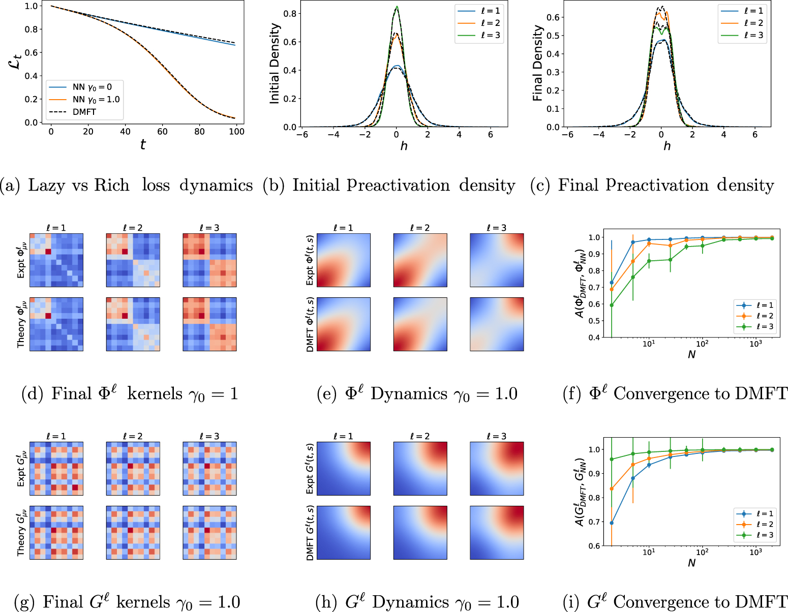
We can derive a similar recursion on the backward pass for $\boldsymbol{G}^{\ell}$'s leading order corrections. Using the same idea from the previous section, we find the following expressions

$$\begin{align*} \boldsymbol{G}^{\ell} = & \left\langle \left[ \dot\phi\left(\boldsymbol{u}_0\right) \boldsymbol{r}_0 \right] \left[ \dot\phi\left(\boldsymbol{u}_0\right) \boldsymbol{r}_0 \right]^{\top} \right\rangle _{\boldsymbol{u}_0, \boldsymbol{r}_0} + \frac{\gamma_0^2}{2} \left\langle \dot\phi\left(\boldsymbol{u}_0\right) \dot\phi\left(\boldsymbol{u}_0\right) \right\rangle _{\boldsymbol{u}_0} \odot \boldsymbol{G}^{\ell+1,2} \\ &+ \frac{\gamma_0^2}{2} \frac{\partial^2}{\partial \gamma_0^2 }|_{\gamma_0 = 0} \left\langle \left[ \dot\phi\left(\boldsymbol{h}\left(\boldsymbol{u}_0,\boldsymbol{r}_0,\gamma_0\right)\right) \boldsymbol{r}_0 \right] \left[ \dot\phi\left(\boldsymbol{h}\left(\boldsymbol{u}_0,\boldsymbol{r}_0,\gamma_0\right)\right) \boldsymbol{r}_0 \right]^{\top} \right\rangle _{\boldsymbol{u}_0, \boldsymbol{r}_0} + \mathcal{O}\left(\gamma_0^4\right). \end{align*}$$

This time, we see that $\boldsymbol{G}^{\ell}$ accumulates corrections from succeeding layers through the backward pass recursion.

We can expand the $\boldsymbol{h}^{\ell}$ and $\boldsymbol{z}^{\ell}$ fields around $\boldsymbol{u}^{\ell,0},\boldsymbol{r}^{\ell,0}$ to find the leading order corrections to each feature kernel

$$\begin{align} \boldsymbol{\Phi}^{\ell,2} = & \frac{1}{2} \frac{\partial^2}{\partial\gamma_0^2}|_{\gamma_0 = 0} \left\langle \phi\left(\boldsymbol{h}^{\ell}\left(\boldsymbol{u}_0,\boldsymbol{r}_0,\gamma_0\right)\right) \phi\left(\boldsymbol{h}^{\ell}\left(\boldsymbol{u}_0,\boldsymbol{r}_0,\gamma_0\right)\right)^{\top} \right\rangle _{\boldsymbol{u}_0,\boldsymbol{r}_0 } \nonumber \\ &+ \frac{1}{2} \text{Tr} \left[ \boldsymbol{\Phi}^{\ell-1,2} \left\langle \frac{\partial^2}{\partial \boldsymbol{u}_0 \partial \boldsymbol{u}_0^{\top}} \left[\phi\left(\boldsymbol{u}_0\right) \phi\left(\boldsymbol{u}_0\right)^{\top}\right] \right\rangle _{\boldsymbol{u}_0 } \right]. \end{align} \tag{ P.20 }$$

The first term requires additional expansion to extract the corrections in γ₀ ²

$$\begin{align} \phi\left(\boldsymbol{u} + \gamma_0 \boldsymbol{C}^{\ell} \boldsymbol{g}^{\ell}\right) &\sim \phi\left(\boldsymbol{u}\right) + \gamma_0 \dot\phi\left(\boldsymbol{u}\right) \odot \left[\boldsymbol{C}^{\ell} \boldsymbol{g}^{\ell}\right] + \frac{\gamma_0^2}{2} \ddot\phi\left(\boldsymbol{u}\right) \odot \left[ \boldsymbol{C}^{\ell} \boldsymbol{g}^{\ell} \right]^2 \nonumber \\ &\sim \phi\left(\boldsymbol{u}\right) + \gamma_0 \dot\phi\left(\boldsymbol{u}\right) \odot \left[\boldsymbol{C}^{\ell,0} \boldsymbol{g}^{\ell,0}\right] + \gamma_0^2 \dot\phi\left(\boldsymbol{u}\right) \odot \left[\boldsymbol{C}^{\ell,0} \boldsymbol{g}^{\ell,1}\right] + \frac{\gamma_0^2}{2} \ddot\phi\left(\boldsymbol{u}\right) \odot \left[ \boldsymbol{C}^{\ell,0} \boldsymbol{g}^{\ell,0} \right]^2 \nonumber \\ \dot\phi\left(\boldsymbol{h}^{\ell}\right)\odot \boldsymbol{z}^{\ell} &\sim \dot\phi\left(\boldsymbol{u}\right)\odot \boldsymbol{r} + \gamma_0 \ddot\phi\left(\boldsymbol{u}\right) \odot \left[\boldsymbol{C}^{\ell,0} \boldsymbol{g}^{\ell,0}\right] \odot \boldsymbol{r} + \gamma_0 \dot\phi\left(\boldsymbol{u}\right) \odot \left[\boldsymbol{D}^{\ell,0} \phi\left(\boldsymbol{u}\right)\right] + \mathcal{O}\left(\gamma_0^2\right) \nonumber \\ C^{\ell,0}_{\mu\alpha}\left(t,s\right) & = A^{\ell-1,1}_{\mu\alpha}\left(t,s\right) + \Theta\left(t-s\right) \Delta_{\alpha}^0\left(s\right) \Phi^{\ell-1,0}_{\mu\alpha}\left(t,s\right) \nonumber \\ D^{\ell,0}_{\mu\alpha}\left(t,s\right) & = B^{\ell,1}_{\mu\alpha}\left(t,s\right) + \Theta\left(t-s\right) \Delta_{\alpha}^0\left(s\right) \Phi^{\ell-1,0}_{\mu\alpha}\left(t,s\right) \end{align} \tag{ P.21 }$$

where we used the fact that $\boldsymbol{C}^{\ell,1} = 0$ which follows from the fact that $\Phi^{\ell-1,1} = 0$, and $\Delta^{\ell,1} = 0$. Now, expanding out term by term

$$\begin{align} \boldsymbol{\Phi}^{\ell} = \;& \boldsymbol{\Phi}^{\ell,0} + \gamma_0^2 \left\langle \left[\dot\phi\left(\boldsymbol{u}\right)\odot \left(\boldsymbol{C}^{\ell,0} \boldsymbol{g}^{\ell,0}\right) \right] \left[\dot\phi\left(\boldsymbol{u}\right)\odot \left(\boldsymbol{C}^{\ell,0} \boldsymbol{g}^{\ell,0}\right) \right]^{\top} \right\rangle \nonumber \\ &+\gamma_0^2 \left\langle \left[\dot\phi\left(\boldsymbol{u}\right) \odot \left(\boldsymbol{C}^{\ell,0} \left[\ddot\phi\left(\boldsymbol{u}\right) \odot \left[\boldsymbol{C}^{\ell,0} \boldsymbol{g}^{\ell,0}\right] \odot \boldsymbol{r}\right]\right) \right] \phi\left(\boldsymbol{u}\right)^{\top} \right\rangle + \text{transpose}\nonumber \\ &+\gamma_0^2 \left\langle \left[\dot\phi\left(\boldsymbol{u}\right) \odot \left(\boldsymbol{C}^{\ell,0} \left[\dot\phi\left(\boldsymbol{u}\right) \odot \left[\boldsymbol{D}^{\ell,0} \phi\left(\boldsymbol{u}\right)\right]\right]\right) \right] \phi\left(\boldsymbol{u}\right)^{\top} \right\rangle + \text{transpose}\nonumber \\ &+\frac{\gamma_0^2}{2} \left\langle \left[ \ddot\phi\left(\boldsymbol{u}\right) \odot \left[ \boldsymbol{C}^{\ell,0} \boldsymbol{g}^{\ell,0} \right]^2 \right] \phi\left(\boldsymbol{u}\right)^{\top} \right\rangle + \text{transpose} \nonumber \\ &+ \frac{\gamma_0^2}{2} \text{Tr} \left[ \boldsymbol{\Phi}^{\ell-1,2} \left\langle \frac{\partial^2}{\partial \boldsymbol{u} \partial \boldsymbol{u}^{\top}} \left[\phi\left(\boldsymbol{u}\right) \phi\left(\boldsymbol{u}\right)^{\top}\right] \right\rangle _{\boldsymbol{u} \sim \mathcal{GP}\left(0,\boldsymbol{\Phi}^{\ell-1,0}\right) } \right] + \mathcal{O}\left(\gamma_0^4\right). \end{align} \tag{ P.22 }$$

We see that the corrections for the $\Phi^{\ell}$ kernels accumulate on the forward pass through the final term so $\Phi^{\ell,2} \sim \mathcal{O}(\ell)$. Now we will perform the same analysis for $\boldsymbol{G}^{\ell}$.

$$\begin{align} \boldsymbol{G}^{\ell} = & \left\langle \boldsymbol{g}^{\ell}\left(\boldsymbol{u},\boldsymbol{r}\right) \boldsymbol{g}^{\ell}\left(\boldsymbol{u},\boldsymbol{r}\right)^{\top} \right\rangle _{\boldsymbol{u} \sim \mathcal{GP}\left(0,\boldsymbol{\Phi}^{\ell-1,0}\right) \boldsymbol{r}\sim\mathcal{GP}\left(0,\boldsymbol{G}^{\ell+1,0}\right) } \nonumber \\ &+ \frac{\gamma_0^2}{2} \text{Tr} \left[ \boldsymbol{G}^{\ell+1,2} \left\langle \frac{\partial^2}{\partial \boldsymbol{r} \partial \boldsymbol{r}^{\top}} \left[\left(\dot\phi\left(\boldsymbol{u}\right) \odot \boldsymbol{r}\right) \left(\dot\phi\left(\boldsymbol{u}\right)\odot \boldsymbol{r}\right)^{\top} \right] \right\rangle _{\boldsymbol{u} \sim \mathcal{GP}\left(0,\boldsymbol{\Phi}^{\ell-1,0}\right) \boldsymbol{r}\sim\mathcal{GP}\left(0,\boldsymbol{G}^{\ell+1,0}\right)} \right] + \mathcal{O}\left(\gamma_0^4\right) \nonumber \\ = & \left\langle \boldsymbol{g}^{\ell}\left(\boldsymbol{u},\boldsymbol{r}\right) \boldsymbol{g}^{\ell}\left(\boldsymbol{u},\boldsymbol{r}\right)^{\top} \right\rangle _{\boldsymbol{u} \sim \mathcal{GP}\left(0,\boldsymbol{\Phi}^{\ell-1,0}\right) \boldsymbol{r}\sim\mathcal{GP}\left(0,\boldsymbol{G}^{\ell+1,0}\right) } \nonumber \\ &+ \frac{\gamma_0^2}{2} \boldsymbol{G}^{\ell+1,2} \odot \left\langle \dot\phi\left(\boldsymbol{u}\right) \dot\phi\left(\boldsymbol{u}\right) \right\rangle _{\boldsymbol{u} \sim \mathcal{GP}\left(0,\boldsymbol{\Phi}^{\ell-1,0}\right)} + \mathcal{O}\left(\gamma_0^4\right). \end{align} \tag{ P.23 }$$

We see that, through the second term, the $\boldsymbol{G}^{\ell}$ kernels accumulate on the backward pass so that $\boldsymbol{G}^{\ell,2} \sim \mathcal{O}(L+1-\ell)$. As before the difficult term is the first expression which requires a full expansion of $\boldsymbol{g}^{\ell}$ to second order

$$\begin{align} \boldsymbol{g}^{\ell} &\sim \dot\phi\left(\boldsymbol{u}\right) \odot \boldsymbol{r} + \gamma_0 \dot\phi\left(\boldsymbol{u}\right) \odot \left[\boldsymbol{D}^{\ell,0} \phi\left(\boldsymbol{u}\right) + \gamma_0 \boldsymbol{D}^{\ell,0} \dot\phi\left(\boldsymbol{u}\right) \boldsymbol{C}^{\ell,0} \boldsymbol{g}^{\ell,0} \right] \nonumber \\ &\quad + \gamma_0 \ddot\phi\left(\boldsymbol{u}\right) \left[\boldsymbol{C}^{\ell,0} \boldsymbol{g}^{\ell,0} + \gamma_0 \boldsymbol{C}^{\ell,0} \boldsymbol{g}^{\ell,1}\right] \odot \boldsymbol{r}. \end{align} \tag{ P.24 }$$

From these terms we find

$$\begin{align} \boldsymbol{G}^{\ell} =\; & \boldsymbol{G}^{\ell,0} + \gamma_0^2 \left\langle\left[\dot\phi\left(\boldsymbol{u}\right) \odot \left(\boldsymbol{D}^{\ell,0} \phi\left(\boldsymbol{u}\right)\right)\right] \left[\dot\phi\left(\boldsymbol{u}\right) \odot \left(\boldsymbol{D}^{\ell,0} \phi\left(\boldsymbol{u}\right)\right)\right]^{\top} \right\rangle\nonumber \\ &+\gamma_0^2 \left\langle \left[\ddot\phi\left(\boldsymbol{u}\right) \left(\boldsymbol{C}^{\ell,0} \boldsymbol{g}^{\ell,0}\right)\right] \left[\ddot\phi\left(\boldsymbol{u}\right) \left(\boldsymbol{C}^{\ell,0} \boldsymbol{g}^{\ell,0}\right)\right]^{\top} \right\rangle \nonumber \\ &+\gamma_0^2 \left\langle \left[\dot\phi\left(\boldsymbol{u}\right) \odot \left(\boldsymbol{D}^{\ell,0} \dot\phi\left(\boldsymbol{u}\right) \boldsymbol{C}^{\ell,0} \boldsymbol{g}^{\ell,0}\right)\right] \boldsymbol{g}^{\ell,0} \right\rangle + \text{transpose} \nonumber \\ &+\gamma_0^2 \left\langle \left[ \ddot\phi\left(\boldsymbol{u}\right) \odot \boldsymbol{C}^{\ell,0} \left(\ddot\phi\left(\boldsymbol{u}\right)\odot \boldsymbol{C}^{\ell,0}\boldsymbol{g}^{\ell,0}\right)\right] \boldsymbol{g}^{\ell,0} \right\rangle + \text{transpose} \nonumber \\ &+ \frac{\gamma_0^2}{2} \boldsymbol{G}^{\ell+1,2} \odot \left\langle \dot\phi\left(\boldsymbol{u}\right) \dot\phi\left(\boldsymbol{u}\right) \right\rangle _{\boldsymbol{u} \sim \mathcal{GP}\left(0,\boldsymbol{\Phi}^{\ell-1,0}\right)} + \mathcal{O}\left(\gamma_0^4\right). \end{align} \tag{ P.25 }$$

Now the correction to the NTK has the form

$$\begin{align} \boldsymbol{K}^{\mathrm{NTK},2} = \boldsymbol{\Phi}^{L,2} + \sum_{\ell = 1}^{L-1} \boldsymbol{G}^{\ell,0} \boldsymbol{\Phi}^{\ell,2} + \sum_{\ell = 1}^{L-1} \boldsymbol{G}^{\ell,2} \boldsymbol{\Phi}^{\ell,0} + \boldsymbol{G}^{1,2} \odot \left( \boldsymbol{K}^x \otimes \boldsymbol{1} \boldsymbol{1}^{\top}\right). \end{align} \tag{ P.26 }$$

Since each $\Phi^{\ell,2}, G^{L+1-\ell,2} \sim \mathcal{O}(\ell)$, each of the two sums from $\ell \in \{1,\ldots ,L-1\}$ gives a depth scaling of the form $\sim \sum_{\ell = 1}^{L-1} \ell = \frac{L(L-1)}{2}$. Since the original NTK has scale $\boldsymbol{K}^{\mathrm{NTK},0} \sim \mathcal{O}(L)$, the relative change in the kernel is $\frac{|\boldsymbol{K}^2|}{|\boldsymbol{K}^0|} = \mathcal{O}(\gamma_0^2 L)$. In a finite width N, network, our definition $\gamma = \gamma_0 \sqrt{N}$ would indicate that a width N network would have corrections of scale $\gamma_0^2 L = \frac{\gamma^2 L }{N }$ in the NTK regime where $\gamma = \mathcal O_N(1)$ provided the network is sufficiently wide to disregard initialization dependent fluctuations in the kernels.