


Abstract
High-power microwave beams used for heating and current drive in magnetically confined fusion plasmas can be broadened significantly by plasma turbulence, negatively impacting the efficiency of the machine. The dependence of this beam broadening on plasma and beam parameters is not yet fully understood, particularly where the dependence on one parameter is not separable from the dependence on the other parameters, meaning the dependence must be expressed via functions of linear combinations of parameters, rather than functions of single parameters. The aim of this work is to develop an empirical model for how the broadening depends on plasma and beam parameters, allowing for the easy estimation of beam broadening by turbulence without the need for computationally expensive full-wave simulations. In this paper, a microwave beam is simulated propagating through a turbulent layer of plasma using the 2D full-wave cold plasma code EMIT-2D. The dependence of beam broadening on background plasma density, fluctuation amplitude, turbulence correlation lengths in the radial and poloidal direction, thickness of the turbulence layer, and microwave beam waist are considered. The parameter scans are conducted in pairwise combinations of the parameters in order to determine the separability of the dependencies. We find that the dependence on the radial and poloidal correlation lengths are not separable from each other, and neither are the dependences on the fluctuation level and the background density, but all other dependencies are separable. Ignoring this inseparability in the correlation lengths will usually result in an over-prediction of the broadening in tokamak plasmas. An empirical formula for the beam broadening based on the turbulence and beam parameters is found for fusion-relevant scenarios, making prediction of the effect possible in microseconds, instead of the hours required for full-wave simulation. This could then be of use for integrated modelling of heating and current drive systems.
Export citation and abstract BibTeX RIS

Original content from this work may be used under the terms of the Creative Commons Attribution 4.0 license. Any further distribution of this work must maintain attribution to the author(s) and the title of the work, journal citation and DOI.
1. Introduction
In magnetically confined fusion devices, microwaves are often used in diagnostic tools and to inject power into the plasmas for the purposes of heating [1, 2], non-inductive start-up [3, 4], and current drive [5]. In conventional tokamaks, global heating and current drive can be achieved via a range of mechanisms, including ion cyclotron resonance heating, neutral beam injection, and electron cyclotron resonance heating. Localized electron cyclotron current drive (ECCD) can also be used to stabilize MHD instabilities such as neoclassical tearing modes [6]. Microwave techniques have the advantages of requiring less space on the vessel wall due to a small launching antenna which can be placed far away from the plasma without loss of efficiency, and the gyrotrons used to generate the microwaves can be housed outside the bio-shield.
In order to inject power, microwave beams must cross the plasma boundary, a region where density fluctuation levels can reach 100% on length scales comparable to that of the microwave wavelength [7]. These fluctuations cause scattering of incident microwaves, leading to the broadening of microwave beams travelling through the plasma. For ITER-like scenarios, it has been predicted that this broadening could result in the doubling of the beam width compared to if no turbulence was present [8]. This broadening has the potential to significantly impact the efficiency of both global and local power injection via microwave beams. It's therefore important to be able to predict this effect when designing and running microwave power injection systems. Whilst full-wave simulations can achieve this, their computational expense makes them impractical when a wide range of plasma and launch scenarios are considered. The determination of the parametric dependence of this broadening could allow the effect to be accounted for in integrated modelling and optimisation studies for future tokamaks in a way that is computationally cheap.
There has been previous investigation of this effect, including development of analytical models for both O-mode [9] and X-mode [10]. This approach has the benefit of allowing for very fast prediction of beam broadening based on plasma and beam parameters, making it ideal for optimisation studies or inter-shot analysis. However, these models rely on methods which will not be applicable in the case of strong turbulence locally creating plasma densities close to or even above the cut-off density in the wave's path, meaning that they will not always be applicable for some fusion relevant scenarios.
Beam broadening has also been investigated using ray tracing methods where the scattering effect is described using a Fokker–Planck solver [8, 11, 12]. There have also been studies using a beam tracing code based on the wave kinetic equation, incorporating the effect of turbulence via a scattering operator derived under the Born approximation [13]. However, these methods are also valid only within certain limits, such as when the turbulence amplitude is small compared to the cut-off density, or when the refractive index does not vary over length scales that are small compared to the wavelength.
In order to simulate particular fusion relevant scenarios where the turbulent scale length is comparable to the microwave wavelength and the fluctuation level is high, directly simulating the beam path through turbulent plasma using full-wave codes is often required. Using this method, 1D parameter scans have previously been carried out [14]. However, the range of parameters is yet to be extended to encompass fusion relevant scenarios. Furthermore, it has not been previously investigated if the impact of changing one parameter is independent of changes in other parameters i.e. if the dependencies are 'separable' as defined in section 2.6.
The work presented here investigates how the broadening of microwave beams by a layer of turbulent plasma depends on plasma and beam parameters. The parameter ranges were set to cover fusion relevant scenarios such as beams used for ECCD, including ranges where turbulence scale length is comparable to microwave wavelength, and fluctuation level is as high as 50%. We considered pairwise combinations of parameters to determine whether the dependence on each parameter is independent of the others and conducted a point-wise fit to the data-set in order to determine an empirical formula for the beam broadening. By determining the dependence of broadening on turbulence and beam parameters in fusion relevant scenarios, a predictive model can be developed which does not require full-wave simulations but is still applicable in parameter regimes that are not analytically tractable. This would be of great use in development of future tokamaks by allowing the quick prediction of beam broadening, and could be incorporated into an integrated model used to optimise heating and current drive efficiency. It could also be used to make predictions on timescales useful for inter-shot analysis as well as real-time predictions based on plasma measurements.
2. Simulation set-up
2.1. EMIT-2D
EMIT-2D is a 2D full-wave, cold plasma code [15, 16]. It uses a finite difference time domain (FDTD) scheme [17] to solve Maxwell's equations (1) and (2) with a cold plasma response equation (3) on a 2D Cartesian grid with absorbing boundary conditions:
where c is the speed of light, ε0 is vacuum permittivity, e is the elementary charge,  is the mass of an electron, and the electron plasma frequency,
  , where n is the electron number density. In equation (3) B0 is the background magnetic field, and it is assumed that there is no background electric field or current density. The equation is then linearised in terms of perturbed quantities. It is also assumed that there are no finite temperature effects, and neglects the contribution of the ions due to their slow response time. The code is therefore valid only in cold plasmas where wave frequencies are sufficiently high, and background electric field and current density are sufficiently small. This is a remarkably good approximation for fusion reactor conditions unless we are close to a resonance.
2.2. Launched beam
The code launches a 2D Gaussian beam. The z-direction is the direction of propagation and the background magnetic field points in the y-direction. In order to excite the beam, a soft-source antenna is used where the field added is given by:
where w0 is the beam waist radius at the focal point, z is the distance along the beam path, and r is the distance from the beam centre. The beam waist radius along the beam line is given by:
and is defined as the distance from the beam centre at which the electric field amplitude falls to  of its peak value. R(z) is the radius of curvature of the wave fronts and
  is the Guoy phase.
By setting B0 to point in the y-direction, we launched an X-mode beam in vacuum. We kept the normalized field strength constant throughout the simulation domain at  where
where  is the electron cyclotron frequency.
2.3. The turbulent density profiles
We chose to study the influence of the following key parameters: background density, fluctuation level, turbulence structure size, width of the turbulence layer, and beam waist. The fluctuations were only in the density profiles, making the turbulence purely electrostatic.
To launch the beam in vacuum, we transitioned the density from zero to its constant background value via a hyperbolic tangent function. In the constant background density region, we transitioned the fluctuation level from zero to a constant value via the same hyperbolic tangent function, before transitioning it back to zero. Though this sharp increase in density is not necessarily realistic for fusion plasmas, we decided that introducing a pedestal like background density would increase the dimensionality of the problem too much. As such, this simplified approach was taken. By considering the simulations run through background density profiles, we were able to determine that this sharp increase in density did not perturb the beam. An example of the background density profile and fluctuation envelope, with an image of a turbulent snapshot are shown in figure 1.
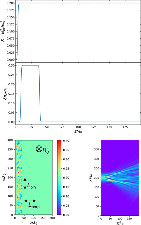
Figure 1. Example ensemble average background density profile and fluctuation level envelope (top), an example turbulent density profile (bottom left) and the RMS electric field (bottom right) of a microwave beam propagating through it. The simulation domain is given in vacuum wavelengths. The colour represents the normalised density  (bottom left) and the RMS field strength in arbitrary units (bottom right). Arrows are marked on to indicate the direction of the background field as well as the direction in which the two different turbulence correlation lengths are defined.
Download figure:
Standard image High-resolution imageThe simulation domain shown in figure 1 is in 2D. This is an acceptable simplification as the turbulent structures are elongated along field lines [7], making the scattering in the toroidal direction small compared to the radial and poloidal direction. The simulation domain is therefore approximately equivalent to a poloidal cross-section in a tokamak.
The turbulent density profile shown in figure 1 represents a snapshot of the plasma. In reality, the plasma would be moving at a speed significantly slower than the wave speed. This allows us to make the assumption that the turbulence is 'frozen', and the overall effect on the beam can be calculated by averaging over an ensemble of turbulence profiles.
In order to generate an ensemble of turbulent density profiles, we used synthetic turbulence. This allowed full control over the turbulence parameters and, for the large number of profiles needed, was less computationally demanding than fluid turbulence generation from a turbulence code.
The density fluctuations were generated using a truncated sum of Fourier-like modes given by [18]:
where Aij
are the amplitudes of the modes, and  are independent random phases uniformly distributed between 0 and 2π.
The amplitudes are related to the structure size by [18]:
where  and
and  , ax
and az
are the box size, and
, ax
and az
are the box size, and  and
and  are the turbulence correlation lengths in the x and z directions respectively. Within the geometry of the simulations, the correlation length perpendicular to the beam path is
  , and the correlation length bi-normal to the beam path and the background magnetic field is
  . In a tokamak scenario, these correspond approximately to the radial and poloidal correlation lengths respectively for perpendicular injection along the radial coordinate.
We generated an ensemble of twenty turbulence profiles for each combination of turbulence correlation lengths. We then scaled the turbulence to the required fluctuation amplitude, applied an envelope function to achieve the required turbulence layer thickness, and added it to the background density. Any negative density values were truncated to zero, resulting in the negative fluctuation amplitude being slightly lower than the positive fluctuation amplitude.
2.4. Calculating beam broadening
In order to determine the broadening, Γ, for each combination of parameters in a scan, we found the ensemble average RMS electric field ( ) at the back-plane of the simulation for each turbulent snapshot. We then calculated the ensemble average of these
  profiles for the ensemble of turbulence snapshots, and compared it to a beam which propagated through an equivalent background profile with no turbulence present. For all simulations, we used an ensemble size of 20 uncorrelated turbulence profiles. This was sufficient for the centre of the broadened beam to align closely with the background case. An example of this is shown in figure 2. This approach results in a statistical uncertainty on the broadening value given by the standard error of the ensemble.
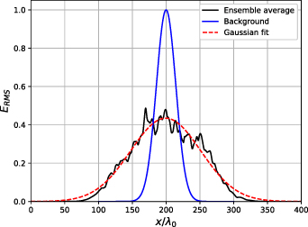
Figure 2. An example of the RMS electric field at the back-plane of the simulation domain, after travelling through the turbulent layer, averaged over an ensemble of 20 uncorrelated turbulence profiles. This is the 'base case' as defined in table 1. A Gaussian fit to the ensemble average is performed and compared to the background Gaussian beam to find the broadening factor.
Download figure:
Standard image High-resolution imageTable 1. Parameters that are varied, how they are varied, and the 'base' value each parameter takes in scans where it is not varied. Note that the background density is only varied through nine values instead of ten, as at the timescales needed for higher densities, the stability condition proved prohibitively computationally expensive.
| Parameter | Varied as | Min | Max | Step | Base |
|---|---|---|---|---|---|
| Perpendicular correlation length |

| −1.5 | 3.0 | 0.5 | 2.0 |
| Binormal correlation length |

| −2.5 | 2.0 | 0.5 | 2.0 |
| Beam waist radius |

| 2.5 | 25.0 | 2.5 | 20.0 |
| Fluctuation level |

| 0.05 | 0.50 | 0.05 | 0.30 |
| Background density |

| 0.05 | 0.45 | 0.05 | 0.20 |
| Width of turbulence layer |

| 5 | 50 | 5 | 30 |
2.5. Parameter scans
The parameters we investigated are listed in table 1, with the value they take in the 'base case' included in every parameter scan, and the ranges they are varied over. All parameters are normalised. Length scales are normalised to the vacuum wavelength, λ0, background density is normalised to the O-mode cut-off density  , and fluctuation amplitude is normalised to background density. We varied the turbulence correlation lengths logarithmically, as we anticipated that broadening will be much smaller when the ratio between correlation length and wavelength becomes either small or large, as seen in previous work [14]. We therefore wanted to treat the ratio symmetrically, which is done by varying its logarithm.
From previous work in the field, we expected scattering to be maximal when the correlation lengths are close to the vacuum wavelength, and to decrease as correlation length moves from this value in either direction [14].
For low density gradients we expected scattering to increase quadratically with fluctuation amplitude [10, 12, 14]. We also expected it to increase with background density and width of the turbulence layer [10, 14]. For the microwave beam waist, we expected an initial increase followed by a gradual decrease, as seen in previous studies [14]. This is due to the dependence of the microwave beam width on its initial waist varying similarly non-monotonically, as can be seen from equation (5).
In order to determine the separability of the dependence on each of these parameters, we carried out a series of 2D scans considering each of the pairwise combinations. Each of these 2D scans required 100 ensembles of 20 simulations to be run, each at an approximate computational cost of 80 CPU hours.
2.6. Fitting
To determine the dependence of the broadening,  , on each parameter and confirm the separability of the dependencies, we performed point-wise fits to the data-set from each 2D parameter scan.
By separable dependence we mean that, for two parameters a and b, the overall broadening can be expressed as a product of two independent functions, f and g, such that:

Within the context of a point-wise fit, the broadening for a particular combination of parameters can then be calculated as:

where C is a normalisation factor, fixing the value of the 'base case' broadening to be  . To allow for the possibility that the dependence is not separable, we included a rotation of co-ordinate axis in the fit, adding an additional fit parameter, θ. The fit parameters fi
and gj
then depend on
. To allow for the possibility that the dependence is not separable, we included a rotation of co-ordinate axis in the fit, adding an additional fit parameter, θ. The fit parameters fi
and gj
then depend on  and
and  as:
as:
As each parameter was varied across ten values, for each 2D parameter scan this resulted in 20 fitting parameters for 100 data points. The exception is scans where background density is varied where, due to computational constraints, only nine values were included. This is owing to the fact that the size of the simulation domain required increases for increased broadening, and that the wave speed in higher density plasma decreases, making the simulations take significantly longer to run. It would be possible to expand upon the range included here, but for this work they were deemed computationally too expensive.
Once a θ value was found for each 2D scan, we knew which dependencies were separable and which were not. We then performed a point-wise fit to the whole data-set, only allowing for inseparability where it had been found.
3. Parametric dependence
Performing the fits to the 2D scans individually, the only pairwise combinations where we found the dependence to be inseparable were those for  vs
vs  , and for
  vs
vs  .
.
An example plot of a 2D dependence of Γ on a pair of separable parameters ( vs
vs  ) is shown in figure 3. Plots of the 2D dependence of Γ on both pairs of inseparable parameters (
 vs
vs  and
and  vs
vs  ) are shown in figures 4 and 5 respectively.
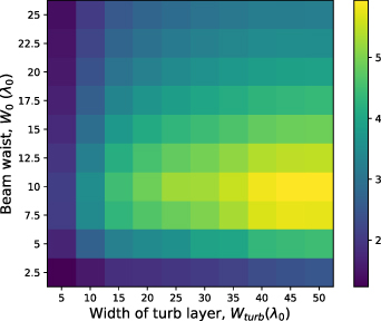
Figure 3. Dependence of broadening on microwave beam waist ( ) and width of the turbulence layer(
 ). Colour represents broadening factor compared to a beam propagating through the same background density profile, with no turbulence present.
Download figure:
Standard image High-resolution image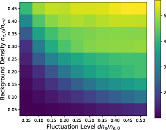
Figure 4. Dependence of broadening on background density ( ) and fluctuation amplitude (
 ). Colour represents broadening factor compared to a beam propagating through the same background density profile, with no turbulence present. From this we see that broadening increases with both background density and fluctuation amplitude, and the tilted nature indicates the dependence is not separable.
Download figure:
Standard image High-resolution image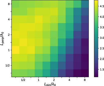
Figure 5. Dependence of broadening on turbulence correlation length in the direction perpendicular to the magnetic field ( ) and in the direction binormal to both the magnetic field and direction of beam propagation (
 ). Colour represents broadening factor compared to a beam propagating through the same background density profile, with no turbulence present. From this we see that both correlation lengths affect broadening differently, and the tilted nature indicates the dependence is not separable.
Download figure:
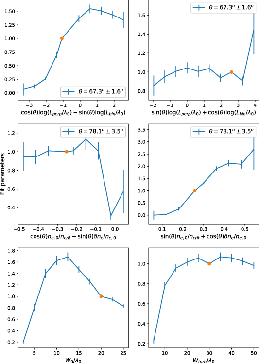
Standard image High-resolution imageThe results of a global pointwise fit, as described in section 2.6, are shown in figure 6. These show how the broadening depends on each parameter (or linear combination of parameters in the cases was the dependence is not separable). It should be noted that for the linear combinations of parameters, the extremal points only correspond to one ensemble of simulations. Every other point corresponds to multiple ensembles. This is why the errors on the extremal points are noticeably larger.
Figure 6. The normalised dependence of broadening on each parameter considered. For the case where the dependence of two parameters is not separable, the dependence on a linear combination of those parameters is shown instead. The orange points correspond to the base value of each parameter, which was used in scans where other parameters were varied. The fit parameters are normalised to this point. The solid lines serve as a guide to the eye.
Download figure:
Standard image High-resolution image
The uncertainty in the broadening measurements from the simulations comes from the standard error on the ensemble average  . There is also an uncertainty associated with the standard error on the ensemble average correlation lengths, fluctuation level, and background density. This contributes to the error on the fit parameters, given by their covariance.
From figure 6, we can see that there is only a weak dependence on the sum of the logarithms of the correlation lengths and a stronger dependence on their difference. This corresponds to having a stronger dependence on the ratio  , meaning that having a larger
  compared to
  increases broadening. In fusion relevant plasmas, the poloidal correlation length (which corresponds to
  ) is usually longer than the radial correlation length (which corresponds to
  ). This would result in less broadening. This rough trend matches the analytical result that (in the low fluctuation level limit) broadening is proportional to
  [10].
[10].
We can also see that the linear combination of  and
and  based on their difference has a weaker effect on the broadening than the linear combination based on their sum. This suggests tha perhaps a key consideration is the peak density of
  and how close it is to a cut-off. Due to the parameter ranges chosen, most points of the scan are outside of the limit where analytical theory can be applied, where we find the dependence of
  and
and  is no longer separable and the broadening no longer scales with
  as predicted by theory [10].
The form of the dependence on microwave beam waist matches that found in [14], where, as  is increased, there is first a sharp increase in the broadening, followed by a gradual decrease. We believe this is due to the dependence of beam width on
  even in the case where turbulence is not present, which can be seen in equation (5).
Finally, the dependence of beam broadening on width of turbulence layer shows that as  increases, so does broadening, until it reaches a maximal value and appears to level off. We believe this is due to a kind of saturation effect, where the beam can no longer become any broader without simply appearing as background noise.
The functional form of the dependence of broadening on plasma and beam parameters, based on separability of parameters, is then:
The numerical values of these fit parameters can be found in
4. Conclusions and further work
We used a 2D full-wave code to simulate microwave beams propagating through turbulent plasma density profiles to determine the dependence of the beam broadening on plasma and beam parameters. We carried out a series of 2D scans in order to identify which dependencies were separable. We found that the dependencies on  and
and  were not separable from each other, and neither were the dependencies on
  and
and  . We found that all other dependencies were separable. We then found the dependence of each parameter, or linear combination of inseparable parameters, by means of a point-wise fit to the whole data-set.
Where applicable, agreement with previous studies was found. However, it would be beneficial to compare this to other methods such as the analytical models [9, 10], ray tracing simulations [8, 11, 12], and beam tracing simulations [13, 18] in order to determine the regions of agreement and disagreement.
The inseparability of the dependence of broadening on the two turbulence correlation lengths is an important result. Currently when simulating beam broadening in fusion relevant scenarios it is common only to have good data for the correlation length in one direction, resulting in both correlation lengths being set equal to each other. This has the potential to significantly under or over predict the broadening of the microwave beam. The sensitivity of broadening to correlation length emphasises the need for diagnostic tools which can measure turbulence parameters to high degrees of precision. For example, from figure 5 the effect of uncertainty in correlation length measurement can be seen. If we take an example where only  is measured, and for simulation purposes the correlation length are set equal to each other despite
  , the broadening would be over-predicted by a factor of 1.2 resulting in a large error on the predicted deposition profile.
A detailed understanding of the parametric dependence of beam broadening on plasma and beam parameters also introduces the possibility of being able to use beam broadening as a turbulence diagnostic. For example, if the other parameters are known well enough, the ratio of the turbulence correlation lengths could be deduced from the measured beam broadening.
Using the parameter dependencies provided here, it should now be possible to predict how much a beam will be broadened by without further simulation, given the scenario falls within the parameter ranges investigated here. This can be done almost instantaneously, rather than the hours that would be required for an ensemble of full-wave simulations to be carried out. This ability to rapidly predict beam broadening could allow for its inclusion in integrated modelling and calculation during experiment.
Acknowledgments
One of the authors (LAH) was funded by the EPSRC Centre for Doctoral Training in Science and Technology of Fusion Energy Grant No. EP/L01663X. This work used the ARCHER UK National Supercomputing Service, allocated through the Plasma HEC (EP/R029148/1), the ARCHER2 UK National Supercomputing Service, allocated through TDoTP (EP/R034737/1), the Cirrus UK National Tier-2 HPC Service at EPCC funded by the University of Edinburgh and EPSRC (EP/P020267/1), and the MARCONI Tier-0 system. Simulations were also conducted on the Viking Cluster, which is a high performance compute facility provided by the University of York. We are grateful for computational support from the University of York High Performance Computing service, Viking and the Research Computing team. This work has been carried out within the framework of the EUROfusion Consortium, funded by the European Union via the Euratom Research and Training Programme (Grant Agreement No. 101052200— EUROfusion). Views and opinions expressed are however those of the authors only and do not necessarily reflect those of the European Union or the European Commission. Neither the European Union nor the European Commission can be held responsible for them.
Appendix: Table of results
Here, we include the parameters from the fit as described in the paper. The results are presented in a table A1. In order to find the predicted broadening, a value of each f as defined in equation (11) should be chosen. These are then multiplied together and multiplied by  before being added to 1 in order to find the factor by which the beam is broadened, such that:

Table A1. Look up table for beam broadening by plasma turbulence based on plasma and beam parameters. p is the parameter (or combination of parameters where the dependence is not separable), f is the value of the fit function, and e is the error on that fit.  ,
,  ,
,  ,
,  ,
,  , and
, and  .
.
| p1 | f1 | e1 | p2 | f2 | e2 | p3 | f3 | e3 | p4 | f4 | e4 | p5 | f5 | e5 | p6 | f6 | e6 |
|---|---|---|---|---|---|---|---|---|---|---|---|---|---|---|---|---|---|
| 0.10 | 0.1 | 0.2 | 0.26 | 0.9 | 0.2 | −0.48 | 0.9 | 0.2 | 0.06 | 0.0 | 0.2 | 2.5 | 0.20 | 0.03 | 5 | 0.23 | 0.03 |
| 0.15 | 0.12 | 0.04 | 0.40 | 0.95 | 0.07 | −0.41 | 0.94 | 0.08 | 0.12 | 0.03 | 0.02 | 5.0 | 0.81 | 0.06 | 10 | 0.78 | 0.04 |
| 0.24 | 0.26 | 0.03 | 0.64 | 1.01 | 0.06 | −0.35 | 1.01 | 0.06 | 0.18 | 0.25 | 0.07 | 7.5 | 1.40 | 0.09 | 15 | 0.96 | 0.04 |
| 0.38 | 0.70 | 0.06 | 1.00 | 1.04 | 0.06 | −0.25 | 1 | − | 0.26 | 1 | − | 10.0 | 1.62 | 0.08 | 20 | 1.02 | 0.05 |
| 0.48 | 1 | − | 1.57 | 1.01 | 0.07 | −0.22 | 1.01 | 0.05 | 0.30 | 1.32 | 0.06 | 12.5 | 1.69 | 0.08 | 25 | 1.06 | 0.05 |
| 0.95 | 1.36 | 0.07 | 2.48 | 1.04 | 0.05 | −0.15 | 1.1 | 0.2 | 0.36 | 1.9 | 0.1 | 15.0 | 1.47 | 0.07 | 30 | 1 | − |
| 1.49 | 1.54 | 0.08 | 3.90 | 0.94 | 0.05 | −0.09 | 1.0 | 0.1 | 0.42 | 2.1 | 0.2 | 17.5 | 1.25 | 0.05 | 35 | 1.07 | 0.05 |
| 2.35 | 1.51 | 0.08 | 6.13 | 1 | − | −0.02 | 0.31 | 0.05 | 0.48 | 2.1 | 0.2 | 20.0 | 1 | − | 40 | 1.06 | 0.04 |
| 3.70 | 1.43 | 0.08 | 9.65 | 0.91 | 0.05 | −0.04 | 0.6 | 0.3 | 0.54 | 2.7 | 0.9 | 22.5 | 0.95 | 0.04 | 45 | 1.03 | 0.04 |
| 5.82 | 1.3 | 0.2 | 15.2 | 1.4 | 0.3 | − | − | − | − | − | − | 25.0 | 0.83 | 0.03 | 50 | 0.98 | 0.04 |