

Abstract
Objective. The day-to-day variability of electroencephalogram (EEG) poses a significant challenge to decode human brain activity in EEG-based passive brain-computer interfaces (pBCIs). Conventionally, a time-consuming calibration process is required to collect data from users on a new day to ensure the performance of the machine learning-based decoding model, which hinders the application of pBCIs to monitor mental workload (MWL) states in real-world settings. Approach. This study investigated the day-to-day stability of the raw power spectral density (PSD) and their periodic and aperiodic components decomposed by the Fitting Oscillations and One-Over-F algorithm. In addition, we validated the feasibility of using periodic components to improve cross-day MWL classification performance. Main results. Compared to the raw PSD (69.9% ± 18.5%) and the aperiodic component (69.4% ± 19.2%), the periodic component had better day-to-day stability and significantly higher cross-day classification accuracy (84.2% ± 11.0%). Significance. These findings indicate that periodic components of EEG have the potential to be applied in decoding brain states for more robust pBCIs.
Export citation and abstract BibTeX RIS
1. Introduction
Electroencephalogram (EEG)-based passive brain-computer interfaces (pBCIs) aim to monitor unintentional changes in users' mental states (Aricò et al 2016, Arico et al 2017, Gao et al 2021) and have gained considerable attention for their potential applications. One of the primary applications of pBCIs is real-time mental workload (MWL) monitoring, which relies on EEG data to provide an objective and non-invasive measure of mental states. This approach is beneficial in safety-critical work environments, such as industrial, transportation, and medical contexts, where hazardous incidents can occur due to a lack of attention or excessive workload (Zander and Kothe 2011, Matthews et al 2015, Dehais et al 2020). Recent years have seen significant efforts to develop machine learning frameworks for classifying MWL based on various EEG features. This work has deepened our neurophysiological understanding of MWL and offers promising avenues for real-time applications (Roy et al 2013, Muhl et al 2014, Arico et al 2016, Lotte et al 2018).
Previous studies have reported significant results in EEG-based estimation of MWL using non-cross-day cross-validation methods (Lim et al 2010, Ayaz et al 2012, Borghini et al 2014, Bagheri and Power 2020). However, brain oscillatory activities fluctuate over time (Dinstein et al 2015), leading to day-to-day variability in the associated EEG features. There may be differences in the pattern of EEG features across days, even when participants are in strictly the same experimental conditions. Therefore, brain decoding models that achieve superior classification using non-cross-validation methods may not generalize well to practice. Inter-day non-stationarity is a critical factor that negatively affects the performance and usability of pBCIs and other BCI paradigms (Shen and Lin 2019). This drawback is particularly evident for pBCIs, which rely on training data with larger sample sizes and more complex experimental settings. In summary, inter-day non-stationarity is a significant challenge for pBCIs, which requires the development of more robust machine learning algorithms and finding features of day-to-day stability to improve the performance and usability of such systems. More reliable and efficient pBCIs for various applications will be possible by overcoming this challenge.
The day-to-day variability of EEG features and its negative impact on machine learning performance has been studied but not adequately addressed in the last decade. Christensen et al found that the performance of EEG-based MWL classification decreases as the time interval between training and test data increases and even drops to chance level while using a cross-day cross-validation manner (2012). Some studies have attempted to tackle the effect of day-to-day variability by collecting training data from multiple days or developing more effective machine-learning methods (Lin et al 2017, Lin 2020, Wu et al 2020). Roy et al compared EEG-based MWL assessment using spectral markers and event-related potentials (ERPs) and found that the ERP-based approach provided stable and efficient workload estimation, outperforming the spectral markers method (2016). Deep learning-based methods have also shown promise in building more generalizable EEG-based mental state decoding models. For example, Hefron et al used a deep recurrent neural network to address the day-to-day variability in estimating MWL from EEG, improving classification accuracy (Hefron et al 2017). Yin and Zhang developed an adaptive stacked denoising AutoEncoder to tackle the cross-day MWL classification task. In their approach, the weights of the shallow hidden neurons are adaptively updated during the testing procedure, leading to a promising performance in cross-day classification (2017).
Despite many research efforts to improve cross-day classification performance, the robustness of classification models still needs to improve. One of the solutions for developing pBCIs that can generalize over time is to find EEG features with day-to-day stability. However, current studies have not fully assessed the day-to-day stability of EEG features. Power spectral density (PSD) features of EEG oscillations are commonly used in pBCIs due to their real-time acquisition convenience. Recent studies demonstrated that PSD can be decomposed into periodic and aperiodic components, and the properties of these two components are distinct, possibly indicating different neural generators. Gerster et al (2022). This decomposition helps to remove confounding factors and allows for a deeper investigation of the relationship between PSD components and brain functions, in contrast to conventional PSD analysis.
Inspired by the idea of parameterizing neural power spectra (Donoghue et al 2020), this study evaluated the day-to-day stability of EEG features extracted from the raw PSD and its periodic and aperiodic components in MWL estimation. We hypothesized that the raw PSD and their periodic and aperiodic components would respond differently to variations in MWL and time. The EEG data were recorded during a visuomotor task under different conditions of the MWL on two different days. Two-way repeated measure ANOVA and intraclass correlation coefficient (ICC) were employed to evaluate the day-to-day variability of these features. Moreover, we compared the cross-day MWL classification performance of machine learning models using different features and validated our results with a public dataset. The main contribution of this paper is twofold. First, we evaluated the day-to-day stability of the raw PSD, periodic, and aperiodic components, which lays the foundation for selecting features with day-to-day stability. Second, we utilized the periodic component to enhance the cross-day MWL classification performance without a calibration phase, thereby enhancing the practicality of pBCIs.
2. Materials and method
2.1. Datasets
We conducted an experiment to collect EEG data and evaluated the day-to-day stability as well as the cross-day classification performance of different features. In addition, we validated the classification results of various features using a public dataset.
2.1.1. Self-collected dataset
The study involved 19 graduate students (12 females), who received financial compensation for their participation. Participants ranged in age from 21 to 27 years (M = 23.8 years, S.D. = 1.18). None of the individuals were pregnant, on medication, or reported known fatigue-related problems. Participants were asked not to consume alcohol the night before the experiment and to abstain from caffeine on the morning of the test. The study was conducted in accordance with the principles embodied in the Declaration of Helsinki. All participants provided their written informed consent before the experiment. The experimental procedure was approved by the Ethics Committee of Tianjin University.
The experimental task for this study utilized the Multi-Attribute Task Battery II (MATB-II) software (Comstock Jr and Arnegard 1992). Three subtasks, namely system monitoring, tracking, and resource management, were employed as components of the MATB. The difficulty of these three subtasks was adjusted to modulate MWL at two levels (low/high). All participants underwent MATB-II training before the formal experiment until performance reached asymptote with minimal error. In this study, participants were asked to complete two sessions (Day 1 and Day 2) separated by more than 48 h. Each session consisted of four randomly assigned blocks, including two blocks of low-load tasks and two blocks of high-load tasks. Each block included a 3-minute rest period followed by a 5-minute MATB task, as depicted in figure 1.

Figure 1. Experimental procedure. Each block consisted of a 3 min eyes-open resting and a 5 min MATB task. Each session consisted of four blocks, including two low-load blocks and two high-load blocks, and the order of the four blocks was randomized.
Download figure:
Standard image High-resolution imageThe EEG signals were recorded at a sampling rate of 1000 Hz throughout the experiment using the NeuroScan NuAmps 64-channel amplifier. We recorded 60 channels of EEG data using the international 10-20 electrode system. Impedance levels were maintained below 5 kΩ to ensure accurate signal acquisition. The right mastoid electrode served as the online reference. All data processing and analyses were performed using EEGLAB Toolbox functions (Delorme and Makeig 2004) and additional scripts developed in MATLAB 2020b® (The MathWorks, Natick, MA). The EEG data were re-referenced to the average of the left and right mastoids, band-pass filtered between 0.1 and 100 Hz, and downsampled to 250 Hz. Visual inspection was used to eliminate muscle artifacts, followed by an independent component analysis (Jung et al 2001) to remove blink and muscle artifacts.
2.1.2. Public dataset
We used a public EEG dataset (Hinss et al 2023) to validate the cross-day classification performance of different features. The dataset comprises recordings of 29 participants' resting state and MATB tasks on three days. We used data from the first and second days. Following the expanded 10–20 system localization, EEG recordings were obtained using 64 active Ag-AgCl electrodes (ActiCap, Brain Products GmbH) and an ActiCHamp amplifier (Brain Products GmbH). The data was sampled at 500 Hz. To improve the reproducibility of the analysis, we preprocessed the raw dataset with the Harvard Automated Processing Pipeline for Electroencephalography (HAPPE) (Gabard-Durnam et al 2018). The preprocessing parameters, feature extraction process, and classification methods were consistent with our data.
2.2. Feature extraction and FOOOF decomposition
The continuous EEG was split into 10 s segments with a 1 s overlap. PSDs were then calculated for each segment using the Welch method, which involved applying Hann-windows of 2 s with a 50% overlap. To parameterize the raw PSD, we used the FOOOF method (Donoghue et al 2020) to decompose the power spectrum into periodic and aperiodic components. Thus, we obtain the raw spectrum and the spectra of two components with a frequency resolution of 1 Hz. Then, the power of the two components and the original spectrum were averaged over the canonical frequency bands, specifically theta (4–7 Hz), alpha (8–13 Hz), low beta (14–20 Hz), high beta (21–30 Hz), and gamma (31–40 Hz) (Newson and Thiagarajan 2018), as shown in figure 2.

Figure 2. FOOOF decomposition. Decompose each raw PSD into periodic and aperiodic components. The algorithm starts by fitting a combination of Gaussian-shaped peaks to the spectral data, identifying the frequencies and amplitudes of the dominant oscillatory activities in the signal. Once the algorithm establishes the peaks, it calculates the 1/f-like background component that explains the non-oscillatory behavior.
Download figure:
Standard image High-resolution imageWe computed grand-averaged PSD brain topographic maps for three types of PSD features, including raw PSD, periodic components, and aperiodic components. These maps were averaged across all participants per condition, which consisted of three MWL levels and two days. In addition, we show the spectra of three types of features on different days and MWL states in typical channels FZ and OZ. After considering previous research and the statistical results of our study, we identified the region of interest for each frequency band associated with the MWL. We then calculated the mean PSD across channels for each condition in these regions of interest.
2.3. Statistical analyses
Two-way repeated measure ANOVAs (2 d × 3 MWLs) were used to examine changes in three types of PSD features across days for each channel. False discovery rate correction (Benjamini and Hochberg 1995) was applied to all p-values to account for multiple tests. In addition, we performed two-way repeated measures ANOVAs (2 d × 3 MWLs) followed by a post hoc paired t-test for the regions of interest associated with each frequency band. All statistical analyses were performed using the EEGLAB Matlab toolbox. We employed three different p-value thresholds: p < 0.05, p < 0.01, and p < 0.001. This approach allowed us to assess the degree of evidence against the null hypothesis at varying levels of rigor.
Next, we examined the test-retest reliability of the features to evaluate day-to-day stability. As defined by (Elliott et al 2020), test-retest reliability refers to the reproducibility of results from a given measure under nearly equivalent conditions. A common statistic used to assess test-retest reliability is the ICC, typically defined as the ratio of the variance of interest to the sum of the variance of interest plus error (Shrout and Fleiss 1979, McGraw and Wong 1996). We calculated the ICC to assess the sensor-level day-to-day stability of three types of features (raw PSD, periodic components, and aperiodic components) of each frequency band (60 channels). In other words, ICC calculations were implemented for each channel in the PSD brain topography to obtain spatially specific reliability estimates. Furthermore, we calculated the ICC and their 95% confidence intervals of the averaged PSD across channels for the region of interest in each frequency band. Additionally, (Koo and Li 2016) recommend using a two-way combined-effects model and an absolute agreement definition for test-retest reliability studies, which is consistent with our experimental design. The ICC calculation formula was as follows,
where  represents the mean square for rows,
  represents the mean square for columns, and
  represents the mean square error. We used ICC statistics with thresholds of ICC > 0.90 indicating excellent stability, ICC > 0.75 indicating good stability, and ICC > 0.50 indicating moderate stability levels (Koo and Li 2016).
2.4. Cross-day classification of PSD-based features
We assessed the performance of four types of PSD-based features in cross-day classification. These included the raw PSD, the periodic feature, the aperiodic feature, and a combination of periodic and aperiodic features. Unlike statistical analysis that focuses on regions of interest, we used data from all channels to construct our classification model. The raw PSD, periodic, and aperiodic features had 300 dimensions (60 channels × 5 frequency bands). In contrast, the combined periodic and aperiodic features encompassed 600 dimensions (60 channels × 5 frequency bands × 2). Each one-dimensional component represented the power in a specific frequency band of one electrode. Periodic features came from the periodic components in the PSD, while aperiodic features came from the aperiodic components. We performed binary-class (rest vs. task) and 3-class (rest vs. low MWL vs. high MWL) classifications using the support vector machine method, implemented in the Matlab machine learning toolbox. The RBF kernel was used, and we optimized the parameters through grid optimization (Cortes and Vapnik 1995).
In contrast to the cross-validation method that uses samples from all days, we did cross-day cross-validation using one day's data as the training set and the other day's data as the test set. The performance was evaluated using the classification accuracy, the area under the curve of the receiver operating characteristic (ROC AUC), and the confusion matrix. The ROC AUC results were considered excellent for AUC values between 0.9 and 1, good for AUC values between 0.8 and 0.9, fair for AUC values between 0.7 and 0.8, poor for AUC values between 0.6 and 0.7 and failed for AUC values between 0.5 and 0.6 (Obuchowski 2003). Additionally, to investigate the classification performance using other classifiers, we reported classification results using linear discriminant analysis, naive Bayes, decision tree, and Adaboost.
2.5. Cross-day feature separability index (CFSI)
To quantitively measure both the stability across days and the separability across mental states, we defined a CFSI. The formula was as follows, where the numerator describes the separability of the features and the denominator expresses the day-to-day variability of the features,
Here, we assumed that the data set  contained
  samples with labels,
  . Each sample was an
  -dimensional feature vector. Dividing the sample set
  into
into  clusters according to the labels
  , where
  was the number of days and
  was the number of classes of features. We defined the feature separability index (FSI) as:
where  represented the centroid of cluster
  ,
,  represented the Euclidean distance between two samples,
  represented the average Euclidean distance of all samples within cluster
  from the centroid
  . The centroid is defined as the arithmetic mean position of all the points in the cluster. The FSI indicated the average distance between all the different classes within the same day. A larger FSI value meant a greater separability of the features. In addition, we defined the day-to-day variability index (DDVI) as:
it indicated the average distance between days for the same class, and the smaller the DDVI value, the lower the day-to-day variability of the feature. A higher index can be obtained when feature separability is high and day-to-day variability is low.
3. Result
3.1. Statistical results of PSD-based features
The averaged PSD of all participants in each condition was shown in supplementary figure 1. The results of two-way repeated measures ANOVAs (2 d × 3 MWL levels) on the raw PSD, periodic components, and aperiodic components were presented in figure 3. For the raw PSD, significant differences in theta band power in the prefrontal midline region and alpha band power in the left and right parietal regions were observed only at the MWL level. Additionally, significant differences in low beta, high beta, and gamma band powers were observed at both time and MWL levels, but without any interaction. Similar to the raw PSD results, the theta and alpha powers for the aperiodic components showed significant differences only at the MWL level, while differences in high beta and gamma powers at the time level were concentrated in the left and right parietal and occipital regions. In contrast, for the periodic components, significant differences in band powers were observed only at the MWL level, with no significant differences at the time level and no interaction. Furthermore, to compare the differences between the three types of PSD-based features on different days, the power spectra of typical channels FZ and OZ are shown in figure 4.

Figure 3. Two-way repeated measures ANOVA results for PSD-based features. A two-way repeated-measures ANOVA was performed on the power spectral values of each channel in each frequency band, and a two-way repeated-measures ANOVA was performed on the power spectral values of each channel in each frequency band. Time factor: Day 1 vs. Day 2, MWL levels Factor: rest vs. low MWL vs. high MWL. We set the FDR-corrected p < 0.05 region to white. The color scales denote F values from ANOVA tests.
Download figure:
Standard image High-resolution image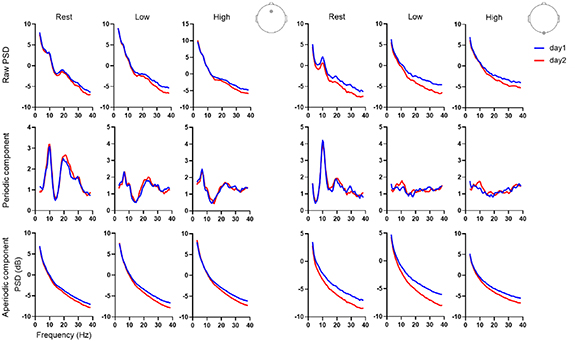
Figure 4. The power spectra of FZ and OZ. The graph on the left displays the results obtained from the FZ channel, while the graph on the right displays the results obtained from the OZ channel. When examining the spectral curves of FZ and CZ electrodes, the main differences between day 1 and day 2 are noticed in the raw PSD and aperiodic components.
Download figure:
Standard image High-resolution imageFigure 3 was mainly intended to show the spatial distribution of the statistical results for the three PSD-based features at the channel level, and for further analysis, we selected regions with p < 0.01 (F value > 8.29) and typical regions associated with MWL (Gevins and Smith 2000, Antonenko et al 2010) as regions of interest for the analysis (theta: mid-frontal region, alpha: bilateral parieto-occipital region, low beta: central parietal region, high beta: central parietal region, gamma: parieto-occipital region). Tables 1–3 show the results of the two-way repeated-measures ANOVA for the regions of interest, and figure 5 shows the results of the post-hoc tests with the channels included in each region.

Figure 5. Two-way repeated measures ANOVA post-hoc test for the region of interest. Two-tailed paired t-test., *p < 0.05. **p < 0.01. ***p < 0.001. ns, not significant.
Download figure:
Standard image High-resolution imageTable 1. Results of two-way repeated-measures ANOVA for regions of interest in the five frequency bands of raw PSD.
| Time | MWL | Interaction | |||||||
|---|---|---|---|---|---|---|---|---|---|
| Band | F | p | Partial η2 | F | p | Partial η2 | F | p | Partial η2 |
| Theta | 0.093 | 0.763 | 0.005 | 16.204 | <0.001 | 0.473 | 1.588 | 0.218 | 0.081 |
| Alpha | 1.031 | 0.323 | 0.054 | 2.474 | 0.098 | 0.120 | 1.086 | 0.348 | 0.056 |
| Low Beta | 1.214 | 0.284 | 0.063 | 8.009 | 0.001 | 0.308 | 0.058 | 0.943 | 0.003 |
| High Beta | 6.291 | 0.021 | 0.259 | 4.032 | 0.026 | 0.183 | 0.351 | 0.705 | 0.019 |
| Gamma | 15.397 | <0.001 | 0.461 | 4.152 | 0.023 | 0.187 | 0.737 | 0.485 | 0.039 |
Table 2. Results of two-way repeated-measures ANOVA for regions of interest in the five frequency bands of periodic component.
| Time | MWL | Interaction | |||||||
|---|---|---|---|---|---|---|---|---|---|
| Band | F | p | Partial η2 | F | p | Partial η2 | F | p | Partial η2 |
| Theta | 0.375 | 0.547 | 0.020 | 22.850 | <0.001 | 0.559 | 0.035 | 0.965 | 0.002 |
| Alpha | 3.973 | 0.061 | 0.180 | 18.231 | <0.001 | 0.503 | 0.652 | 0.527 | 0.035 |
| Low Beta | 4.303 | 0.052 | 0.192 | 12.394 | <0.001 | 0.407 | 0.414 | 0.663 | 0.022 |
| High Beta | 2.044 | 0.169 | 0.102 | 25.780 | <0.001 | 0.588 | 2.846 | 0.071 | 0.136 |
| Gamma | 3.725 | 0.069 | 0.171 | 18.192 | <0.001 | 0.502 | 1.183 | 0.317 | 0.061 |
Table 3. Results of two-way repeated-measures ANOVA for regions of interest in the five frequency bands of aperiodic component.
| Time | MWL | Interaction | |||||||
|---|---|---|---|---|---|---|---|---|---|
| Band | F | p | Partial η2 | F | p | Partial η2 | F | p | Partial η2 |
| Theta | 0.039 | 0.845 | 0.002 | 20.281 | <0.001 | 0.529 | 2.047 | 0.143 | 0.102 |
| Alpha | 1.629 | 0.218 | 0.083 | 16.748 | <0.001 | 0.482 | 1.189 | 0.316 | 0.062 |
| Low Beta | 2.271 | 0.149 | 0.112 | 5.877 | 0.004 | 0.261 | 0.779 | 0.466 | 0.041 |
| High Beta | 9.632 | 0.006 | 0.348 | 2.271 | 0.117 | 0.112 | 0.945 | 0.398 | 0.049 |
| Gamma | 13.752 | 0.001 | 0.433 | 2.567 | 0.090 | 0.124 | 1.204 | 0.311 | 0.062 |
For raw PSD, the theta and low beta bands were only affected by the MWL factor and not by the time factor, the alpha band was not significantly different under either factor, and the high beta and gamma bands were significantly different under both factors, but there was no interaction effect (table 1). For the periodic component, the power of each band differed significantly only at the level of MWL and did not differ significantly across days (table 2). For the aperiodic components, both theta, alpha, and low beta bands were influenced by MWL factors only, while high beta and gamma were influenced by time factors (table 3).
3.2. ICC results for PSD-based features
The ICC of the theta band in the prefrontal theta, high beta, and gamma bands in the parieto-occipital region of the periodic component was larger than that of the raw PSD and the aperiodic component (figure 6). Table 4 illustrates the ICC of the average PSD of the region of interest in five different frequency bands (theta: mid-frontal region, alpha: bilateral parieto-occipital region, low beta: central parietal region, high beta: central parietal region, gamma: parieto-occipital region). The ICCs of the five bands of the region of interest for the periodic component were all greater than 0.7, except for the alpha band in the low (ICC = 0.62, CI95 = 0.25–0.83) and high (ICC = 0.61, CI95 = 0.24-0.83) MWL states.
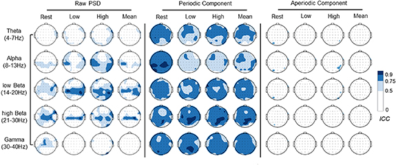
Figure 6. The topography of ICC for each frequency band. ICC across two days of three types of features among each frequency band. 'Mean' represented the average ICC across MWL levels. The ICC of the five bands of the periodic component was higher than 0.75 in some brain regions, whereas the ICC of all five bands of the aperiodic component was less than 0.5.
Download figure:
Standard image High-resolution imageTable 4. ICC of the region of interest in the five frequency bands. LB represented the lower bound of the 95% confidence interval and UB represented the upper bound.
| Raw PSD | Periodic components | Aperiodic components | ||||||||
|---|---|---|---|---|---|---|---|---|---|---|
| Band | MWL | ICC | LB | UB | ICC | LB | UB | ICC | LB | UB |
| Theta | Rest | 0.10 | −0.36 | 0.53 | 0.70 | 0.36 | 0.87 | 0.16 | −0.32 | 0.57 |
| Low | 0.38 | −0.09 | 0.71 | 0.87 | 0.69 | 0.95 | 0.31 | −0.18 | 0.67 | |
| High | 0.34 | −0.15 | 0.68 | 0.84 | 0.63 | 0.93 | 0.20 | −0.29 | 0.60 | |
| Alpha | Rest | 0.52 | 0.11 | 0.78 | 0.93 | 0.84 | 0.97 | 0.55 | 0.16 | 0.80 |
| Low | 0.75 | 0.47 | 0.90 | 0.62 | 0.25 | 0.83 | 0.63 | 0.26 | 0.84 | |
| High | 0.47 | 0.03 | 0.76 | 0.61 | 0.24 | 0.83 | 0.48 | 0.03 | 0.76 | |
| Low Beta | Rest | 0.69 | 0.37 | 0.87 | 0.85 | 0.65 | 0.94 | 0.69 | 0.35 | 0.87 |
| Low | 0.87 | 0.62 | 0.95 | 0.84 | 0.54 | 0.94 | 0.54 | −0.01 | 0.82 | |
| High | 0.83 | 0.61 | 0.93 | 0.80 | 0.57 | 0.92 | 0.37 | −0.04 | 0.69 | |
| High Beta | Rest | 0.85 | 0.66 | 0.94 | 0.81 | 0.56 | 0.92 | 0.67 | 0.32 | 0.86 |
| Low | 0.80 | 0.47 | 0.92 | 0.92 | 0.80 | 0.97 | 0.57 | 0.06 | 0.83 | |
| High | 0.73 | 0.43 | 0.89 | 0.93 | 0.84 | 0.97 | 0.42 | 0.02 | 0.72 | |
| Gamma | Rest | 0.59 | 0.21 | 0.81 | 0.88 | 0.71 | 0.95 | 0.73 | 0.42 | 0.89 |
| Low | 0.52 | 0.00 | 0.80 | 0.87 | 0.67 | 0.95 | 0.56 | −0.03 | 0.83 | |
| High | 0.28 | −0.16 | 0.64 | 0.92 | 0.81 | 0.97 | 0.38 | −0.03 | 0.70 | |
3.3. Cross-day classification results of PSD-based features
In our data, periodic features achieved the highest classification accuracy in binary (84.2% ± 11.0%) and three-class (58.9% ± 11.5%) classification tasks. This performance was significantly superior to that of raw PSD features, which yielded accuracy rates of (69.9% ± 18.5%, t18 = 4.064, p < 0.001, Cohen's d = 0.932) and (52.7% ± 14.0%, t18 = 2.161, p = 0.044, Cohen's d = 0.496) in binary and three-class classifications, respectively. Additionally, consistent results were obtained in the public dataset. Periodic features exhibited the highest classification accuracy of (93.8% ± 4.6%), significantly outperforming raw PSD features at (73.4% ± 25.4%, t18 = 4.471, p < 0.001, Cohen's d = 0.830). Figure 7 shows the averaged classification accuracy across all subjects.
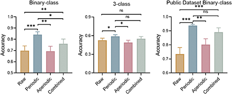
Figure 7. Classification accuracy results. 'Combined' stands for the combined feature of periodic and aperiodic features, paired t-test, *p < 0.05. **p < 0.01. ***p < 0.001. ns, not significant. Binary-class: Rest vs. Task, 3-class: Rest vs. Low MWL vs. High MWL. Compared with the raw PSD features, periodic features for cross-day binary classification improved the accuracy by 14.3% in our dataset and 20.4% in a publicly available dataset, achieving 84.2% and 93.8% accuracy, respectively.
Download figure:
Standard image High-resolution imageMoreover, to examine the performance of the classification model based on periodic components versus other models, figure 8 shows the results of the ROC AUC analysis. Classifiers trained by periodic feature had the highest ROC AUC in binary and 3-class classification. There was no significant difference in the ROC AUC for the four types of features, and all of them reached the level of 'good' or 'excellent'. To provide more details on the classification results than just the accuracy, as shown in figure 9, we plotted a confusion matrix to visualize the performance of different classification models. The periodic component feature had better performance than other features in identifying the rest and task states. However, in the 3-class classification results, the periodic component, like the other features, performed poorly in distinguishing between high and low MWL. The ROC AUC and confusion matrix results for the public dataset are shown in supplementary figures 2 and 3.
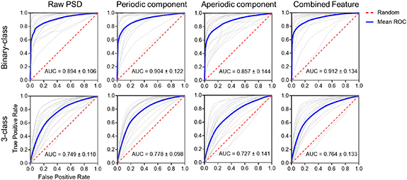
Figure 8. ROC curves of binary and 3-class classifications. The gray line in the figure represents the ROC AUC curves of different subjects, and the blue line represents the average ROC AUC curve. Each curve in the lower right triangle does not perform as well as random guessing. The curve appearing in the upper left of the ROC has a better performance classification.
Download figure:
Standard image High-resolution image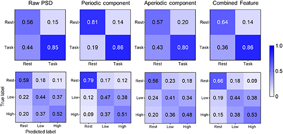
Figure 9. Confusion matrix of binary and 3-class classifications. Each row shows the distribution of instances in the real class. Similarly, each column shows the instances in the prediction class. The periodic component feature had better performance than other features in identifying the rest and task states. However, in the 3-class classification results, the periodic component, like the other features, performed poorly in distinguishing between high and low MWL.
Download figure:
Standard image High-resolution image3.4. Results of CFSI
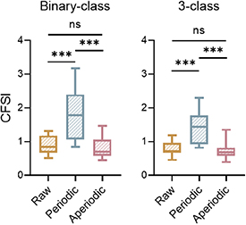
To further investigate the reason for the superior performance of periodic components in cross-day classification, we proposed the CFSI. It evaluated the cross-day separability of features by calculating the distance between the centroids of sample sets with different MWLs on the same day divided by the distance between the centroids of sample sets with the same MWLs on different days. A higher index can be obtained when feature separability is high and day-to-day variability is low. As shown in figure 10, the CFSI of the periodic component feature was higher than that of the raw PSD feature (t18 = 3.664, p = 0.001, Cohen's d = 0.840) and the aperiodic component feature (t18 = 4.276, p < 0.001, Cohen's d = 0.981) in the results of binary classification. Consistent with the binary classification results, the periodic component feature outperformed the other features in the 3-class classification (raw PSD vs. periodic component: t18 = 3.687, p = 0.001, Cohen's d = 0.846; aperiodic component vs. periodic component: t18 = 4.984, p < 0.001, Cohen's d = 1.143). In addition, we also did a statistical analysis of the numerator (FSI) and denominator (DDVI) of the CFSI separately, and the results are shown in supplementary figure 4.
Figure 10. CFSI results. paired t-test, *p < 0.05. **p < 0.01. ***p < 0.001. ns, not significant. The CFSI for periodic features was significantly higher than the raw PSD (t18 = 3.664, p = 0.001, Cohen's d = 0.840) and aperiodic components (t18 = 4.276, p < 0.001, Cohen's d = 0.981) in the binary classification results, and the same results were obtained in the 3-class classification (raw PSD vs. periodic component: t18 = 3.687, p = 0.001, Cohen's d = 0.846; aperiodic component vs. periodic component: t18 = 4.984, p < 0.001, Cohen's d = 1.143).
Download figure:
Standard image High-resolution image
4. Discussion
This study investigated the day-to-day variability of PSD features and their periodic and aperiodic components in evaluating MWL. Furthermore, we examined the viability of using periodic features to improve cross-day MWL classification performance. The experimental results showed that the periodic components exhibited high day-to-day stability and achieved better cross-day MWL classification performance without a calibration phase. This finding not only promised to improve the usability of pBCIs for MWL estimation but also opened up possibilities for decoding other brain states in future applications.
4.1. Day-to-day variability of the periodic and aperiodic components of the PSD
Aperiodic activity in the power spectrum varied from day to day, as demonstrated by changes in the slope of the 1/f curve. Figures 3 and 4 show that aperiodic activity differed between two days across all levels of MWL. Specifically, variations from day to day were noticeable in the beta and gamma bands, whereas the theta and alpha bands showed minimal fluctuations. The region most affected by day-to-day variability was the parieto-occipital region. To our knowledge, the reason why aperiodic activity varies from day to day is unclear yet. Conventionally, the aperiodic activity was considered noise in the frequency domain and often required correction. However, recent studies, such as (Gyurkovics et al 2021) and (Ouyang et al 2020), have suggested that it might have functional significance. Gao et al proposed the aperiodic activity as an estimator of excitation-inhibition (E-I) balance using computational modeling (Gao et al 2017). Furthermore, the aperiodic activity has been related to the integration of the underlying synaptic currents, which have a stereotyped double-exponential shape in the time domain that naturally gives rise to the 1/f-like nature of the PSD (Buzsaki et al 2012). Such day-to-day variability may caused by changes in the excitation/inhibition balance (Turrigiano 2011), continuous interaction and competition among the neuronal populations (Kelly et al 2008), and distributed neuromodulation effects (Marder 2012).
In contrast, the periodic component was stable from day to day. The two-way repeated measures ANOVA (see figure 3) indicated that the periodic components in each frequency band did not show significant variations across days. Conversely, the high beta and gamma bands of the raw PSD and aperiodic components were significantly affected by both time and MWL. The ICC analysis results shown in figure 6 further support these findings. The periodic component's consistency was generally higher than that of the aperiodic and raw PSD components. Notably, the FOOOF method extends the PSD-based MWL feature from the low-frequency band to the high-frequency band. The theta and alpha bands of raw PSD did not differ significantly between days (figure 5). This was consistent with previous findings that selected theta and alpha bands of the raw PSD as stable MWL features rather than high-frequency bands (Brouwer et al 2012, Arico et al 2016). Due to the limitations of the narrow-band PSD extraction method, PSDs in high-frequency bands have rarely been used as MWL features in previous studies. We found that the high beta and gamma bands of the periodic component have good day-to-day stability and can distinguish different MWLs because they strip out the aperiodic component (figure 5).
The observed spatial distribution of the raw PSD differs from that of the periodic components (supplementary figure 1). This suggests that the spatial distribution of the raw PSD may be driven, at least in part, by aperiodic activity, as oscillations above the aperiodic component are not separated. Notably, variations in the spatial distribution of theta and alpha bands in the periodic components under different MWL states recapitulate well-established spatial patterns, with theta power concentrated in the frontal midline and alpha power predominantly distributed over posterior areas. However, the spatial distribution of low beta, high beta, and gamma bands of raw PSD differs significantly from that of the periodic components. For the periodic component, the low-beta band was concentrated in the parietal-occipital midline and the high-beta band over posterior areas, with power decreasing as MWL increased. The power of the gamma band in the parieto-occipital region was almost negligible at rest but increased as MWL levels went up. Furthermore, the spatial distribution of the periodic components varies less across days than the raw PSD.
4.2. The periodic component can improve cross-day classification accuracy
As shown in figure 7, the cross-day classification performance of the periodic component feature was significantly better than the raw PSD feature. Periodic features achieved the highest cross-day classification accuracy in our data and public datasets. This result was consistent with our expectations. Previous results show that MWL can be easily classified using data from the same day (Borghini et al 2014, Aghajani et al 2017). However, the accuracy of the classification model drops when we use test data collected at a different time from the training data. Christensen et al demonstrated that the decline in classification accuracy appears to level off at the hours level and was maintained above chance from one day to up to two weeks later (2012). The variations in PSD-based EEG features from day to day primarily stem from the aperiodic component. Since the raw PSD includes the aperiodic component, training the classifier with raw PSD features leads the classifier to learn not just MWL-related information but also time-dependent patterns. This is a plausible explanation for the lower accuracy observed when using raw PSDs as features for cross-day classification. Moreover, we evaluated the performance of four different feature types on other classifiers (see supplementary tables 1 and 2) and obtained similar results.
The CFSI results (figure 10) show that the periodic component feature outperformed the raw PSD and aperiodic features. Furthermore, the results of the FSI and DDVI can be found in supplementary figure 4. We demonstrated that the day-to-day variability of the periodic feature is significantly lower than that of the raw PSD features (binary-class: t18 = 4.748, p < 0.001, Cohen's d = 1.089; 3-class: t18 = 5.151, p < 0.001, Cohen's d = 1.181), and in contrast, the feature separability is significantly higher than that of the raw PSD (binary-class: t18 = 3.664, p = 0.001, Cohen's d = 0.840; 3-class: t18= 3.687, p = 0.001, Cohen's d = 0.846). Furthermore, our hypothesis was supported by the finding that the day-to-day variability of aperiodic features was significantly higher than that of the raw PSD feature (binary-class: t18 = 4.189, p <0.001, Cohen's d = 0.961; 3-class: t18 = 4.828, p <0.001, Cohen's d = 1.107).
Notably, when we analyzed the day-to-day variability of PSD-based features, we focused on specific regions of interest for our statistical analysis. However, we used data from all channels to construct our classification model. We did this because every channel might have valuable characteristics that can help with classification. Additionally, preprocessing is essential before applying the FOOOF method to extract features. FOOOF extracts features from the PSD curves. It fits Gaussian shapes to the peaks in the spectrum without any prior knowledge of what those peaks represent. Unfortunately, factors like blinking and muscle artifacts can introduce noise into the PSD curve. This noise can lead to unreliable results when extracting periodic components.
4.3. Avoiding the calibration phase of BCI by improving the day-to-day stability of features
The day-to-day variability of PSD-based features has been a significant challenge in the development and practical application of pBCIs. This study suggests that improving the day-to-day stability of features is crucial to avoid BCI calibration. The decoding of MWL states in BCIs is strongly affected by the day-to-day variability of EEG features. Existing classification methods typically require recalibration of the model with new EEG data for each subject, which is time-consuming and inconvenient for users. Compared with the raw PSD features, periodic features for cross-day binary classification improved the accuracy by 14.3% in our dataset and 20.4% in a publicly available dataset, achieving 84.2% and 93.8% accuracy, respectively. This approach can enhance the practicality of PSD-based BCIs without requiring calibration, making them more user-friendly. Notably, the proposed approach of using periodic component features to improve cross-day classification accuracy is not limited to MWL discrimination. Other PSD feature-based classifications, such as emotion recognition, may also benefit from this approach. However, further research is necessary to explore the generalizability of this approach to other brain states.
This study has a few limitations to keep in mind. First, the process of obtaining periodic features involves complex preprocessing, which can make it computationally intensive. This could affect its practical use in real-time classification. Second, EEG data reflects the ever-changing activity of the brain, which can be influenced by various non-cognitive and physiological factors. Despite our best efforts, it is challenging to eliminate the impact of these variables. So, when interpreting our results in the context of MWL assessment literature, it is essential to be cautious.
5. Conclusion
Our study investigated the day-by-day variability and cross-day classification performance of the periodic and aperiodic components of the PSD. Our results suggested that the periodic component is likely to stay consistent from day to day and result in improved cross-day classification performance compared to the raw PSD features and the aperiodic component. Improving the day-by-day stability of the features could reduce the calibration time required for EEG-based systems, thus facilitating the application of pBCIs. These findings have implications for developing pBCIs that can reliably estimate MWL without interfering with the primary task. Furthermore, periodic features have the potential to be applied in decoding other brain states, opening up possibilities for the development of more effective pBCIs.
Acknowledgments
This work was supported by the National Key Research and Development Program of China (No. 2021YFF1200603) and the National Natural Science Foundation of China (Nos. 62276184, 61806141).
Data availability statement
The data that support the findings of this study are openly available at the following URL/DOI: https://doi.org/10.5281/zenodo.8238159.
Supplementary data (0.7 MB PDF)