Abstract
Objective. Finite element modelling has been widely used to understand the effect of stimulation on the nerve fibres. Yet the literature on analysis of spontaneous nerve activity is much scarcer. In this study, we introduce a method based on a finite element model, to analyse spontaneous nerve activity with a typical bipolar electrode recording setup, enabling the identification of spontaneously active fibres. We applied our method to the vagus nerve, which plays a key role in refractory epilepsy. Approach. We developed a 3D model including dynamic action potential (AP) propagation, based on the vagus nerve geometry. The impact of key recording parameters—inter-electrode distance and temperature—and uncontrolled parameters—fibre size and position in the nerve—on the ability to discriminate active fibres were quantified. A specific algorithm was implemented to detect and classify APs from recordings, and tested on six rat in-vivo vagus nerve recordings. Main results. Fibre diameters can be discriminated if they are below 3 μm and 7 μm, respectively for inter-electrode distances of 2 mm and 4 mm. The impact of the position of the fibre inside the nerve on fibre diameter discrimination is limited. The range of active fibres identified by modelling in the vagus nerve of rats is in agreement with ranges found at histology. Significance. The nerve fibre diameter, directly proportional to the AP propagation velocity, is related to a specific physiological function. Estimating the source fibre diameter is thus essential to interpret neural recordings. Among many possible applications, the present method was developed in the context of a project to improve vagus nerve stimulation therapy for epilepsy.
Export citation and abstract BibTeX RIS
1. Introduction
Neuromodulation, defined as the modulation of the nervous system activity with artificial means, is widely used to treat chronic disorders [1]. It can be performed by neurostimulation (the electromagnetic approach to neuromodulation), and more specifically by electrical current pulses delivered through electrodes that activate or inhibit excitable tissues. Clinical applications include deep-brain stimulation for Parkinson's disease [2, 3], peripheral nerves stimulation for bladder incontinence [4, 5] or foot drop [6, 7], and vagus nerve stimulation (VNS) for refractory epilepsy [8–10] to name only a few.
Conventional electrical stimulation delivers pulses in a continuous (or intermittent) fashion, in an 'open-loop'. Recently much attention has been paid to responsive stimulation, where pulses are delivered in response to a physiological feedback acquired by the device, in a 'closed-loop'. For instance, in spinal cord stimulation to treat chronic pain, spinal cord evoked compound action potentials (APs) are used to adjust stimulation pulse [11]. In deep brain stimulation to treat psychiatric illnesses, stimulation is automatically adjusted in response to changes in the patient's electrical brain activity [12]. Many peripheral nerves (dorsal genital nerve, pudendal nerve, S3 afferent nerve roots, S1 and S2 ganglia) have been stimulated as treatment of urinary incontinence and lower urinary tract symptoms, and most of these nerves have also been used as sources of information to detect bladder events to propose a responsive therapy [13]. Acquiring and processing the physiological feedback required for responsive therapy is, however, far from being an easy task. In peripheral nerves, for instance, the signal to noise ratio (SNR) is low and it is difficult to distinguish the desired physiological feedback from other information carried in the nerve bundle [13].
VNS is a widely used neuromodulation treatment for refractory epilepsy. Despite its largely common use, the mechanism of action of VNS is not yet fully elucidated [14, 15]. Nearly one third of patients do not respond to VNS, and very little is known about why this occurs [16, 17]. Today, vagus nerve stimulators operate in either of two stimulation modes, continuous or in a 'closed-loop', where the stimulation is conditional to the occurrence of a seizure. This later mode of stimulation is promising since the abortive effect of VNS has been confirmed by several human and animal studies [18–20]. However, today, the seizure detection used is based on ictal tachycardia [21], even if a significant number of patients do not experience any ictal tachycardia. A more reliable seizure biomarker would therefore be highly valued.
Consequently, a better understanding of the vagus nerve—more specifically regarding its spontaneous activity in the framework of epilepsy—would be beneficial. Indeed, knowing what fibres are active during a seizure or at rest could enable the identification of new seizure biomarkers, providing the physiological feedback required for a responsive therapy. This knowledge also gives insight in the role of the types of nerve fibres in seizure activity, hence contribute to our understanding of their role in epilepsy, suggesting new methods of epilepsy management. Besides, understanding the way nerve activity is captured by the electrodes can help us optimise nerve monitoring systems.
Modelling is a valuable tool to analyse both a nerve spontaneous activity and the mechanisms underlying its response to electrical stimulation. Most reported studies related to the vagus nerve have focused on electrical stimulation [22, 23]. The percutaneous auricular VNS has also been modelled [24, 25]. More specifically [22, 23], aimed to improve the stimulation parameters and reduce side effects. They focused on the potential field generated by the electrodes to selectively target specific types of fibres believed to result in anti-epileptic effects [22, 23]. To the best of our knowledge, no study has modelled vagus nerve spontaneous activity.
Modelling the spontaneous activity of the nerve requires knowledge of both the dynamics (i.e. evolution in time) of AP propagation and its contribution to the electrical potential captured by the electrodes (i.e. 3D modelling). The dynamics of AP propagation has been studied for decades, first in the squid giant axon [26], later adapted to mammals [27]. On the other hand, 3D modelling of nerves usually focused on static (i.e. not time dependent) potential fields [22, 23] thus not integrating the AP propagation.
We found only two teams whose work linked the dynamics of AP propagation with a 3D volume geometry, to model the compound activity recorded in peripheral nerves by a specified set of electrodes. The most detailed model adds the AP of a number of independently firing single fibres to a noise signal [28]. However, in the work of these authors, nodes of Ranvier are modelled by voltage sources and not current sources, and the AP propagates at an arbitrarily chosen velocity (i.e. the AP propagation velocity is not based on the specific fibre model equations). Another study implemented a complex electrode network to focus on a specifically located source to discriminate the activity of a given nerve fascicle against others [29].
In this paper, we present the implementation of a 3D volume conductor model of a nerve using finite elements, including a representation of the propagation of a spontaneous AP. We use this model to analyse the vagus nerve spontaneous activity as recorded with bipolar hook electrodes. We propose a method to infer the AP propagation velocity distribution (and thus the distribution of active fibre diameters) from a given neural recording. We applied our method to analyse the vagus nerve activity recorded in vivo in six rats.
2. Methods
2.1. Surgical procedure
Six male Wistar rats obtained from the local animal facility were used. All rats were provided ad libitum access to food and water under a 12 h day/night cycle. The experimental procedure, described in Stumpp et al [30], has been approved by the University Health Sciences Sector Laboratory Animal Protection Committee (2018/UCL/MD/001).
Animals were anaesthetized with 6% Sevoflurane in pure  at a 3 l min−1 flow rate. As the initial anaesthesia took effect, the Sevoflurane was stopped, and the animals were injected with 60 mg kg−1 Ketamine and 7 mg kg−1 Xylazine intraperitoneally. The level of anaesthesia was controlled by the withdrawal reflex upon noxious paw stimulation and maintained by additional intraperitoneal injections of 60 mg kg−1 Ketamine, approximately every 30 min. The body temperature was controlled via a rectal probe and maintained at 37.5 °C by a heating pad.
To record the vagus electroneurogram (VENG), the left vagus nerve was exposed. Loose perineural connective tissue was removed over a length of 10–15 mm and the exposed nerve was placed on two elevated hook electrodes (with 2 mm inter-electrode distance, see figure 3(b)). The nerve and surrounding tissue were covered with silicone oil (Merck KGaA, Darmstadt, Germany) to prevent dehydration. The surgical procedure is further detailed in [30].
2.2. Recording setup
A custom-made amplifier was used [30]. Hardware filters consist of a bandpass (12–12 000) Hz. The gain of the amplifier is 800 and the observed root mean square noise of the amplifier is 0.5 μV referred to the input. The signal was acquired at 80 kHz via a USB-6212 multifunction I/O-device (National instruments, Austin, USA) for an overall resolution of 0.175 μV bit−1 and a dynamic range of ±3.5 mV, both referred to the input. A custom-made MATLAB R2017a application (MathWorks, Natick, USA) was used to acquire the data. The potentials were recorded in a bipolar differential mode.
The nerve temperature was also measured, since it has an impact on the nerve activity and more specifically on AP propagation velocity. During an acute in-vivo experiment, in a hook setup, the nerve is lifted by the electrodes from its original position. The space between the wound and the nerve is thus air. Analysing the characteristic times of the different mechanisms of heat transport governing the temperature of the nerve—i.e. the heat exchange by conduction and convection between the nerve and the surrounding air medium and the supply of heat by the blood flow—we can show that the temperature of the nerve can be evaluated as the average of equidistant measurements below and above the nerve (see appendix
2.3. Theoretical approach
An AP propagates along the nerve fibres at a velocity  that is a function of the fibre diameter. Two electrodes longitudinally placed along the nerve fibre would see, in a monopolar recording with an external reference, the monopolar AP with a delay
  where
where  is the distance between the electrodes (see blue traces in figure 1). However, the two electrodes are fed into the differential inputs of an amplifier (see red traces in figure 1).
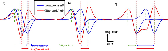
Figure 1. Description of AP. In blue, the individual potential fluctuation seen by each of the electrodes of a longitudinal differential montage referred to the internal membrane potential. In red, the difference between the blue APs, i.e. the differential AP corresponding to the differentially recorded signal. In green, the duration between the peaks of a monopolar AP. (a) Below the spatial aliasing limit (SAF = 0.5). (b) Spatial aliasing limit (SAF = 1). (c) No spatial aliasing (SAF = 2).
Download figure:
Standard image High-resolution imageAs can be seen in figure 1(c), the time between the minimum and the maximum peak ( ) of a differentially recorded AP equals
  if the AP at the first electrode has returned to zero when the second electrode sees the potential. In this case, the velocity can be deduced from the differentially observed duration such as
  .
.
However, if  is below a critical inter-electrode distance value or if
  is above a critical velocity value, then
  differs from
  (figure 1(a)) and
  can no longer be deduced from
  . We refer to this situation as spatial aliasing. In this situation, the duration between the peaks of a monopolar AP, defined as
  (see figure 1, in green), is larger than the time required by the AP to travel from one electrode to the other (
 ) (see figure 1(a)). Therefore, the contribution of the first recording electrode is mixing with the contribution of the second electrode.
We define the duration factor  as the ratio between the two durations:
We define the spatial aliasing factor  as the ratio of
  and
and  , such that spatial aliasing is observed when
  :
:
The critical inter-electrode distance  represents the minimal distance for which no spatial aliasing appears, and is defined as:

In this definition, the fibre diameter associated with the critical distance is defined as the critical fibre diameter.
 and
and  are both related to spatial aliasing but provide complementary information.
  directly quantifies spatial aliasing (it is higher than one when there is little or no spatial aliasing and smaller otherwise). It can be simply deduced (i.e. without the need to refer to a 3D model) for any fibre diameter because
  only depends on the temperature.
  can be seen as a correction factor (that can be equal, less or greater than one), to infer
  from what is observed in a recording, since it directly relates
  (required to calculate
  ) and
) and  (observed in the recording). It depends on the electrode configuration and the 3D geometry.
2.4. Modelling
2.4.1. General overview
The study aims to simulate the single fibre AP propagation in the modelled nerve. The AP is as described by Schwarz's model for myelinated nerve [27], adapted to mammal fibres by Wesselink [31]. These equations provide an estimate of the transmembrane potential and current at any node of Ranvier as a function of time. Variants of the model have been used in several studies [29, 32]. This work focuses on myelinated fibres (A- and B-fibres) rather than unmyelinated fibres (C-fibres). Indeed, since myelinated fibres have larger diameters than unmyelinated fibres, and since the amplitude of an AP is proportional to the square of the fibre diameter [33], the amplitude of APs of myelinated fibres are much larger, leading to a predominant contribution in an in-vivo recoding.
In a further step, the calculated transmembrane current—i.e. the current sources at the nodes of Ranvier—was used as the input for a 3D geometrical and electrical finite element model (FEM) simulation of the vagus nerve. The FEM computed the potential at any point, in particular at the recording electrode positions. The signal expected to be recorded with bipolar electrodes can thus be calculated.
2.4.2. Implementation of AP propagation
The modelling parameters are those of [31], as detailed in appendix
While the transmembrane potential represents the main output of the Hodgkin–Huxley derived equations, the membrane current,  , at a node of Ranvier n, can be calculated as follows for a spontaneous AP (i.e. without external stimulation):
 being the capacitive current from the inside of the fibre,
  being the current though the ionic channels outward from the inside of the fibre,
  being the transmembrane capacity,
  the potential just outside the membrane,
  the internal membrane potential and
  the current through the ionic channels outward from the inside of the fibre, at a node of Ranvier n. Considering Kirchhoff's law at the node n (and between its neighbours n−1 and n + 1) [34]:
where  is the axoplasmic resistance, considered equal between each node of Ranvier.
Such that:
Physical quantities are expressed in SI units.
2.4.3. Finite element model
The vagus nerve geometry was reproduced in a FEM as described by [22] and can be seen in figure 2. It was implemented with the module Electrical Currents of COMSOL Multiphysics 5.5 (COMSOL Inc., Burlington, MA). The fibre geometry was taken from the transverse section of a histology sample, then the nerve was extruded along its length. The diameter of the nerve was 400 μm [35], and the nerve length was long enough to avoid boundary problems when the AP was propagating. Parameters of the layers constituting the nerve were taken from [23]. For the sake of simplicity, during simulations, only one fibre is considered at a time.

Figure 2. Artist view of the model. Layers, from external to internal: connective tissue (gold yellow), endoneurium (yellow), epineurium (pale brown), perineurium (brown), myelin (pale green)—cytoplasm (green). Nodes of Ranvier are short stretches of axon devoid of myelin.
Download figure:
Standard image High-resolution imageEach node of Ranvier is represented as a cylinder. Nodes of Ranvier are the inputs for the FEM. They are current sources defined by equation (6) and not voltage sources as in [28]. These are calculated for each node and each time bin by a MATLAB program, while COMSOL computes the resulting potential distribution based on the implemented geometry. A request is made by COMSOL to MATLAB to load the current sources at specific time bins. The communication between current sources computed by MATLAB and COMSOL request for input current source is realised with a local TCP/IP connection in MATLAB thanks to the LiveLink for MATLAB module from COMSOL.
The AP propagation modelling using Wesselink–Schwarz equations has been extensively studied and validated [31, 36]. The velocity observed in our 3D model was compared to the 1D model from [31] and to measurements based on in-vivo recordings (see [37]).
2.5. Data analysis
2.5.1. General overview
Our method aims to link the spontaneous APs observed during a recording to the spectrum of active fibre diameters. First, the method was assessed through simulations. Simulated APs were compared in several situations (section 2.5.2). The method was assessed in terms of achievable sensitivity and accuracy (section 2.5.3), which were linked to the aliasing phenomenon (introduced in section 2.3). Then, the method was used to infer the diameter of fibres from rat VENG recordings (section 2.5.4).
2.5.2. Illustration of encountered situations
To analyse the impact of one parameter at a time on the recording, different situations were compared, keeping other variables constant:
- different diameters of fibres,
- different positions of the fibre in the nerve section,
- different inter-electrode distances,
- different nerve temperatures.
Unless otherwise stated, the fibre diameter was 5 μm, the temperature was 25 °C as typically observed in the recordings, the inter-electrode distance was 2 mm, the position was central and the fibre—electrodes distance was 0.3 mm.
Four fibre positions were used, as shown in figure 3(a). In a nerve of 200 μm radius, the active fibre was: centred (position 1); placed 100 μm from the centre, both toward the electrodes or in opposite direction to it (positions 2, 3); or placed 100 μm from the centre in the perpendicular direction (position 4).
2.5.3. Inferring the diameter of fibre in simulations
Normalised APs from all fibre sizes at the central position were simulated and used as templates. Normalised APs extracted from the model at the positions of figure 3, with different levels of noise, were compared to these templates. The APs were analysed with an infinite SNR, and SNRs of 6 dB and 3 dB by the addition of white Gaussian noise. The cross-correlations between the tested AP and the templates were calculated. The template with the maximum correlation was associated with the tested AP, providing an estimation of the fibre diameter. The comparisons of positions, with respect to the central position, and of different levels of noise, were realised with an independent Chi-square test, suitable for categorical classification. We only chose to use simulated templates that are corresponding to a fibre in the centre of the nerve, since the fibre position is not expected to significantly affect the AP temporal shape [38]. Changes in absolute amplitude value are taken care of by the normalisation. We have tested the effect of the nerve position within the nerve and found no effect (see section 3.1.2). Moreover, choosing the central fibre position only for the template—rather than many templates corresponding to different fibre position—prevents overfitting.
2.5.4. Inferring the diameter of fibre from rat VENG recordings
Individual spikes expected to correspond to the AP of single fibres were identified in the VENG recordings of each rat. A spike detection algorithm was adapted from [30, 39, 40]. The algorithm works in three steps: (a) spike candidates are detected by convoluting the recording with a generic spike, (b) detected spikes are separated into clusters and isolated spike candidates are rejected, (c) cluster centroids are used for a second detection with narrower detection range to generate the final spike identification. Finally, detected spikes are extracted from the raw signal.
As in section 2.5.3, normalised APs from all fibre sizes at the central position were simulated and used as templates. Spikes detected from the recordings were normalised and compared with the templates. Normalisation annihilates influence of amplitude on the cross-correlation output. A diameter was associated with each detected spike, corresponding to the maximal correlation obtained from the templates comparison. Spikes with a fibre diameter detected as being above the studied range (i.e. 13 μm and above, hence associated with the largest template) were quantified.
3. Results
3.1. Study of model parameters
3.1.1. Influence of the fibre size
The differential APs are displayed in figure 4(a) for three fibre sizes ([2, 5, 9] μm). The 5 μm and 9 μm fibre showed more spatial aliasing than the smaller fibre of 2 μm. This is due to their faster velocity.
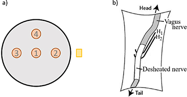
Figure 3. (a) Representation of different fibre positions, not to scale. The brown circles represent the fibres and the yellow rectangle the electrode. (b) Representation of the recording hook electrodes ( ,
,  ) setup [30].
Download figure:
Standard image High-resolution image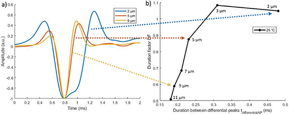
Figure 4. Simulation of bipolar APs for different fibre sizes. (a) Temporal signal. Amplitudes are scaled to their minimum value. (b) Duration factor (DF) as a function of the duration between the differential peaks ( ). Each point represents one fibre size.
Download figure:
Standard image High-resolution imageFigure 4(b) shows the DF of the different fibre sizes. Large fibres were characterised by a smaller duration between the peaks. They were more difficult to differentiate, as seen in section 3.3. Indeed, variations of duration between two diameters become smaller for larger fibres. For example, the duration  of an 11 μm fibre was 95% of the duration of a 9 μm fibre, while the duration of a 3 μm fibre was 65% of the duration of a 2 μm fibre.
3.1.2. Influence of the position of the fibre
As described in figure 3, several positions were studied to evaluate the influence of the fibre position on the recorded signal. Figure 5(a) shows the temporal behaviour of the simulated AP at these positions for a fibre of 5 μm at 25 °C with an inter-electrode distance of 2 mm. Figure 5(b), shows the DF of [11, 9, 7, 5, 3, 2] μm fibres for these positions.

Figure 5. Comparison of simulated APs for different fibre positions, with 2 mm inter-electrode distance, at 25 °C. (a) Temporal signal for a 5 μm fibre. (b) Duration factor (DF) as a function of the duration between the differential peaks ( ). Each point represents one fibre size ([11, 9, 7, 5, 3, 2] μm).
Download figure:
Standard image High-resolution imageDespite a noticeable modification in amplitude, the duration between the peaks  remained similar. Indeed, the peak-to-peak amplitude varied by 60%, whereas duration varied by only 8%. In this regard, fibre diameters can still be discriminated exploiting the temporal signal with little influence of the fibre position.
3.1.3. Influence of the inter-electrode distance
As the inter-electrode distance increases, the AP takes more time to reach the second electrode. Hence, for a given AP velocity, the larger the distance between the electrodes, the smaller the aliasing. This can be visualised on figure 6(a). If the distance is large enough, there is no spatial aliasing ( ), DF is close to 1, and the duration of the peak increases linearly with the distance (see figure 6).
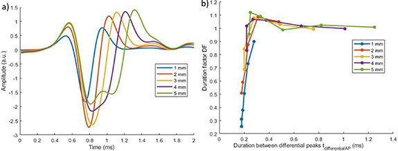
Figure 6. Comparison of simulated for different inter-electrode distances at 25 °C. (a) Temporal signal for a 5 μm fibre. (b) Duration factor (DF) as a function of the duration between the differential peaks ( ). Each point represents one fibre size ([11, 9, 7, 5, 3, 2] μm).
Download figure:
Standard image High-resolution image3.1.4. Influence of the temperature
As the temperature increases, the propagation velocity increases. Taking equation (2), a higher velocity induces a smaller SAF, i.e. more spatial aliasing. Figure 7 shows that the spatial aliasing was more important at higher temperature.
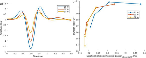
Figure 7. Comparison of simulated APs for different temperatures with 2 mm inter-electrode distance. (a) Temporal signal for a 5 μm fibre. (b) Duration factor (DF) as a function of the duration between the differential peaks ( ). Each point represents one fibre size ([7, 5, 3, 2] μm).
Download figure:
Standard image High-resolution image3.1.5. Evaluation of the spatial aliasing and critical fibre diameter
Critical fibre diameters (defined in section 2.3 as the largest fibre diameter for which there is no spatial aliasing for a given inter-electrode distance), associated with typical inter-electrode distances, were evaluated at several temperatures. At 25 °C, a duration of 0.3 ms for  was observed in the 3D model (
 only depends on the temperature). SAF was calculated at 25 °C and fibres with critical diameter were identified (see figure 8(a)). These were 3 μm and 7 μm, respectively for inter-electrode distances of 2 mm and 4 mm (indicated by an arrow in figure 8(a)). Beyond these diameters, spatial aliasing was observed. The observation of spatial aliasing was also consolidated with the vertical part of the curves (spatial aliasing, for fibres larger than the critical fibre diameter) compared to the horizontal part of the curves (no spatial aliasing). This observation was given at 25 °C but can also be described at other temperatures, for instance at 37 °C as shown on figure 8(b).

Figure 8. Comparison of simulated APs for different inter-electrode distances. (a) At 25 °C. (b) at 37 °C. Each point represents one fibre size ([13, 11, 9, 7, 5, 3, 2] μm). Points targeted by an arrow correspond to the critical fibre diameter.
Download figure:
Standard image High-resolution image3.2. Sensitivity of the model
Simulated AP for fibres located in several positions were classified with the AP templates in the central position. Figure 9 shows that the position of the fibre within the nerve had little effect on diameter prediction accuracy. For fibres larger than the critical fibre diameters, the mean error varied from 0.14 μm ± 1.58 μm to 1.4 μm ± 2.63 μm and no dependence can be established from the position (p > 0.05). For this reason, further analysis focussed on the centrally located fibres, believed to be most representative.
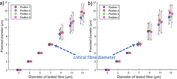
Figure 9. Mean predicted diameter as a function of actual diameter for four fibre positions at 25 °C. The error bars represent one standard deviation. The electrode intercontact distance is 4 mm. (a) SNR = 6 dB. (b) SNR = 3 dB.
Download figure:
Standard image High-resolution imageThe influence of noise on prediction accuracy was analysed (see figure 10). The accuracy decreased with the SNR, as expected. The mean predicted fibre diameter was not dependent on noise (p > 0.05) but the standard deviation was significantly higher when SNR decreased from 6 dB to 3 dB (Levene test, p < 0.05).
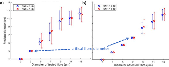
Figure 10. Mean predicted diameter as a function of actual diameter for SNRs of 6 dB and 3 dB at 25 °C. The error bars represent one standard deviation. The inter-electrode distance is 2 mm (a) and 4 mm (b).
Download figure:
Standard image High-resolution imageThe repartition of assigned templates for a given fibre diameter is represented in figure 11 for a SNR of 3 and 6 dB. The accuracy reached 100% for fibre diameters smaller or equal to the critical fibre diameters. The decrease in sensitivity was closely linked to the critical distance. For instance, taking an inter-electrode distance of 2 mm and an SNR of 3 dB (i.e. worst case considered), a fibre of 5 μm (i.e. with spatial aliasing starting to be observed) was assigned to a diameter of 5 μm 84% of the time and to a diameter of 7 μm 16% of the time. The accuracy of classification for fibre diameters larger than the critical fibre diameters decreased to 35%, in the worst case of the considered fibre diameter range (i.e. 9 μm). If one considers acceptable a classification of a fibre within a range of ±2 μm around its real value, then the accuracy increased to 85%.

Figure 11. Repartition of assigned templates for a tested fibre diameter for SNRs of 6 dB (plain lines) and 3 dB (dashed lines) at 25 °C. Depending on the inter-electrode distance: 2 mm (a) and 4 mm (b). The decrease of sensitivity is closely linked with the critical distance and fibres that are beyond the range.
Download figure:
Standard image High-resolution image3.3. Evaluation of the active fibres from in-vivo VENG recordings
Spikes were detected in the spontaneous VENG of the six rats with the adapted detection algorithm (see section 2.5.4). For each detected spike, a comparison of the spike with modelled APs was performed. This allowed us to reconstruct the occurrences of active fibres in the recording. Figure 12(a) presents the mean and standard deviations of occurrences of active fibres that were detected and classified in the recordings. Ninety per cent of the detected spikes were included in the studied range (2–11 μm). A typical example from one recording is given in figure 12(b). Each individual spike classified is displayed in grey and the 3 μm template is displayed in red. The AP amplitudes have been adjusted to better demonstrate any temporal mismatch.
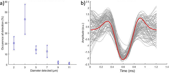
Figure 12. (a) Histogram of occurrence of fibre diameters, based on detected spikes (mean and standard deviation). (b) Typical example of in-vivo detected spikes (grey) associated with a diameter of 3 μm (simulation template in red).
Download figure:
Standard image High-resolution image4. Discussion
In this paper, we developed a detailed 3D model of a propagating AP. We simulated the effects of inter-electrode distance, fibre position across the nerve section, temperature and propagation velocity. Finally, we proposed a method to identify the diameter of the source fibres by comparing recorded APs with a set of simulation templates.
Fibre diameters below the critical fibre diameter can be unequivocally identified based on the bipolar recording. Diameters above this value can still be identified to some extent. The accuracy depends on the inter-electrode distance, temperature and SNR. For instance, the accuracy was above 85% for an inter-electrode distance of 2 mm, an SNR of 3 dB, at 25 °C, considering acceptable a classification of a fibre diameter within a range of ±2 μm. The fibre position within the nerve had no significant effect on the discrimination accuracy. If the inter-electrode distance is increased to 4 mm (and the other parameters kept constant), the accuracy exceeds 90% for the same range of fibres. More generally, our methodology allows to predict the range of fibres that can be discriminated (and the accuracy whiting that range) for a given inter-electrode distance and temperature.
The modification of the recorded AP shape, introduced as spatial aliasing in this paper, was observed with an experimental setup [41]. Thanks to our 3D model, spatial aliasing has been further investigated by characterising its effects in various typical experimental situations.
To the best of our knowledge, a method to detect and classify spontaneously active fibres with a dynamic 3D model in a bipolar setting has never been presented before. Koh et al [29] demonstrated the value of dynamic modelling. In their work, convolutions were used in a spatiotemporal matrix to discriminate fibre positions from activity recorded with a multi-electrode cuff. Our algorithm uses a simpler electrode arrangement (hook) to detect the fibre diameter, rather than position. We believe that both algorithms are complementary.
Fibre diameter discrimination has already been introduced in experiments with velocity selective recording by Taylor et al [42, 43]. Using a multi-electrode cuff and dedicated recording software with adjustable delays, they were able to discriminate fibres based on propagation velocity. The method, like ours, is most sensitive to slower, smaller fibres. Even if the purpose of their work and ours is similar—fibre diameter discrimination—our methodologies strongly differ, and our work is focused on short recording setups using simple hook electrodes, whilst theirs focused on applications where cuffs with multiple contacts are used. Our model provides additional details on the discrimination accuracy, based on the temporal properties of the signals, and we have studied the effect of different parameters to demonstrate their respective importance in the discrimination. Our dynamic 3D model therefore completes the experimental results of [42, 43] based on 1D considerations.
To study the robustness of fibre diameter discrimination in a recording, white Gaussian noise was added to the signal. The levels of noise added to the signal have an amplitude typically observed in our VENG recordings, giving SNRs in agreement with previously published work [44]. Their findings suggest that, for small inter-electrode distances, increasing this distance enhances the SNR, which is concordant with our observations in the recordings.
Our analysis indicated a higher discrimination accuracy for smaller fibres. This is explained by a smaller propagation velocity for smaller fibres. Since the AP has more time to travel from one electrode to the other, contributions to both electrodes are less mixed, the recorded AP is less prone to spatial aliasing, and thus easier to distinguish. However, even if smaller fibres do not suffer from spatial aliasing, they exhibit a smaller AP amplitude, therefore implying a lower SNR (considering the noise level constant), which tends to decrease discrimination accuracy. If the SNR becomes too low, it can be difficult to distinguish an AP from the background, to analyse its waveform and so, a fortiori, to discriminate fibres, even when not suffering from spatial aliasing. Our work did not analyse the impact of fibre diameter on the AP amplitude, and so on the SNR. However, examples of accuracies reached for different values of SNR are given in section 3.2.
As implemented in this work, our method only addresses a limited range of fibre diameters. In particular, the unmyelinated C fibres are not represented despite their importance in the vagus nerve [37]. The main reason is that recording activity in such fibres requires other electrodes than used in our experiments [45, 46]. This does not exclude later applying the same principle to signals obtained with the adequate technical recording but we concentrated first on that part of accessible spectrum where we expect to find activity in relation to known side effects of VNS such as respiratory interference, hoarseness, cough, etc [23, 47]. Fibres responsible for the anti-epileptic effects of VNS are known to pertain to the same myelinated 2.5–8 μm diameter groups as well [23, 48].
One should also consider that our method classifies AP in a recording and counts the number of firings, regardless of whether they come from one single fibre (firing repetitively) or different ones. Since nerve fibres tend to fire repetitively, the histogram of active fibre diameters, based on detected spikes (e.g. figure 12(a)), cannot be directly related to the histology of the nerve. In doing so, the repeated firing would result in an overestimation of the number of fibres anatomically present.
The effect of anaesthetics is another issue deserving attention. While isoflurane is known to reduce the vagus nerve activity [49], the effect of ketamine, which is used in this study, is the subject of debate. A limited effect on the level of activity has been described [50] but it may have an inhibitory effect on the vagus nerve transmission [51]. No significant change was found in sensory nerve conduction velocity. Significant changes in motor nerves found in [52] might be due to temperature shifts. Temperature was controlled in our study (see appendix
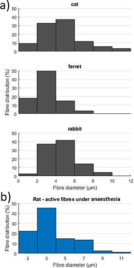
Despite this limitation, some comparison can be made between the histogram of active fibre diameters in rats (as proposed here, see section 3.3) and the histology of the nerve. There is little literature to compare our results with. Histology of the vagus nerve is available for the cat [53], ferret [54], rabbit [55], where similar ranges of diameters are found. Since the fibre distributions are similar in these mammals, we find our results consistent with previous literature (see figure 13).
Figure 13. (a) Diameter-frequency distribution of myelinated fibres in the cervical vagus nerve of a cat [53], ferret [54] and rabbit [55] found in the literature. (b) Diameter-frequency distribution of active fibres under anaesthesia in our study.
Download figure:
Standard image High-resolution image
A main purpose of our work in rats is to develop a method that could be applied later in humans. The goal of the method is to derive information on vagus nerve activity through an electrode placed on the nerve in the frame of VNS [56], for example. Because nerve fibres of different diameters subtend different physiologic functions, an estimation of the diameter of the active fibres is essential to identify physiologic activity from the neural signal. Such recordings are expected to be very important not only in understanding the many physiologic mechanisms to which the vagus nerve participates but also in the frame of clinical questions such as the early detection of seizures [57] or of risk of SUDEP in epilepsy.
Our results are derived from experiments at 25 °C and the model is adaptable to other temperatures; also, the geometry of the nerve can be tuned. Therefore, the model could be adjusted to other species including humans. The findings of this work already implicitly provide suggestions for optimal electrode designs.
5. Conclusion
This study showed the possibility to discriminate the diameter of spontaneously active fibres using a method based on a dynamic FEM model. The impact of experimental parameters—both controlled and uncontrolled—on the method was evaluated. An optimisation of the recording setup was proposed, more specifically regarding the inter-electrode distance, improving discrimination of the fibre diameters. The SNR of the recording was considered in the accuracy evaluation. We believe the proposed method is valuable for research in neurology. More specifically, it could be applied to better understand activity in the vagus nerve to improve VNS therapy for epilepsy.
Acknowledgments
This work has been funded by the Pôle Mecatech of the Walloon Region (Belgium). We are grateful for the help provided by Geoffrey Vanbienne in the realisation of our hardware setup.
Data availability statement
The data that support the findings of this study are available upon reasonable request from the authors.
: Appendix A
To analyse the different phenomena governing the temperature of the nerve, it is represented here as a cylinder of volume V, diameter D ( ), lateral surface S and length L (
 ), surrounded by air and with a flow of blood through it. We also assume that the density and the heat capacity of the nerve are similar to those of liquid water.
Two mechanisms influence the temperature T of the cylinder: the heat exchange with the air (by conduction and convection) and the heat supply by the blood flow through the cylinder.
If the sole heat exchange with the air was taking place, the time evolution of the temperature of the cylinder would be described by the following equation:
where  is the density of liquid water,
  is the heat capacity of liquid water, t is the time,
  is the temperature of the cylinder,
  is the temperature of the surrounding air,
  is the heat transfer coefficient between the cylinder and the surrounding medium.
Consequently, the heat exchange between the cylinder and the surrounding air has the following characteristic time:
Due to the small diameter of the cylinder, we can assume that conduction is the dominant mechanism of heat transfer between the cylinder and the air. Hence,  , with
  the thermal conductivity of the air, taken here equal to
  [58]. Consequently,
  is calculated (using
  ).
).
If the sole flow of the blood in the cylinder was controlling its temperature, the time evolution of the temperature of the cylinder would be described by the following equation:
where  is the blood temperature and
  is flow rate of blood in the cylinder.
Consequently, the heating of the cylinder by the flow of blood into it has the following characteristic time:
Considering that the equivalent diameter of the total flow cross section of the capillaries in the cylinder is  and that the velocity of the blood in a single capillary is
  [59],
[59],  is calculated and, hence,
  .
.
As a conclusion of this short analysis, we see that the characteristic time of heat exchange with the air is much smaller than the characteristic time of blood renewal in the cylinder. Hence, we can reasonably assume that the temperature of the cylinder is the one of the surrounding air.
: Appendix B
The parameters that were used to simulate the single fibre AP propagation in the modelled nerve were initially proposed by Wesselink [31].
B1. Gating Variables


Gating coefficients (a, b) are expressed in terms of  and membrane potential (V) are expressed in terms of
  .
.
B2. Model Parameters
 membrane capacity,
 : leakage conductance,
 sodium permeability,
 : potassium conductance,
 : intra-axonal resistance,
 : leakage equilibrium potential,
 sodium equilibrium potential,
 : sodium concentration outside cell,
 : sodium concentration inside cell,
 : potassium equilibrium potential,
 : resting membrane potential,
 : Faraday constant,
 : gas constant,
 : absolute temperature,
B3. Membrane Currents
 : sodium current (
 )
)
 : (fast) potassium current (
 )
)
 : leakage current (
 )
)
 : total ionic current (
 )
)
 : capacitive current [
 ]
]
 total nodal membrane current (
 )
)