
Abstract
Objective. fMRI-based neurofeedback (NF) interventions represent the method of choice for the neuromodulation of localized brain areas. Although we have already validated an fMRI-NF protocol targeting the facial expressions processing network (FEPN), its dissemination is hampered by the economical and logistical constraints of fMRI-NF interventions, which may be however surpassed by transferring it to EEG setups, due to their low cost and portability. One of the major challenges of this procedure is then to reconstruct the BOLD-fMRI signal measured at the FEPN using only EEG signals. Because these types of approaches have been poorly explored so far, here we systematically investigated the extent at which the BOLD-fMRI signal recorded from the FEPN during a fMRI-NF protocol could be reconstructed from the simultaneously recorded EEG signal. Approach. Several features from both scalp and source spaces (the latter estimated using continuous EEG source imaging) were extracted and used as predictors in a regression problem using random forests. Furthermore, three different approaches to deal with the hemodynamic delay of the BOLD signal were tested. The resulting models were compared with the only approach already proposed in the literature that uses spectral features and considers different time delays. Main results. The combination of linear and non-linear features (particularly the largest Lyapunov exponent and entropy measures) projected into the source space, spatially filtered by independent component analysis (ICA) and convolved with multiple HRF functions peaking at different latencies, increases significantly the reconstruction accuracy (defined as the correlation between the measured and approximated BOLD signal) from 20% (direct comparison with the method used in the current literature) to 56%. Significance. With this pipeline, a more accurate reconstruction of the BOLD signal can be obtained, which will positively impact the transfer of fMRI-based neurofeedback interventions to EEG setups, and more importantly, their dissemination and efficacy in modulating the activity of the desired brain areas.
Export citation and abstract BibTeX RIS

Original content from this work may be used under the terms of the Creative Commons Attribution 4.0 license. Any further distribution of this work must maintain attribution to the author(s) and the title of the work, journal citation and DOI.
1. Introduction
When provided with real-time information about a specific brain process, an individual can attempt to manipulate it through self-regulation, which allows for adjustments in the internal mechanisms used for its manipulation. This process is called neurofeedback (NF) [1, 2]. If the brain process under manipulation is dysfunctional, its regularization through NF is expected to result in behavioral changes [3]. Therefore, clinical applications of NF interventions have been conducted throughout the last years, namely on patients with Attention Deficit/Hyperactivity Disorder (ADHD), depression, addictions, anxiety disorders and other conditions [2, 4, 5].
Electroencephalography (EEG) and functional Magnetic Resonance Imaging (fMRI) are the most commonly used techniques for implementing a NF loop [4]. The different characteristics of each technique led to the development of different approaches for their application in NF studies. In particular, EEG-based NF interventions target mostly attention and relaxation-related EEG rhythms, namely the alpha frequency band, the ratio of theta power over alpha power, or the µ rhythm [5]. Levering its remarkable spatial resolution, NF studies using fMRI target more selective brain regions and/or networks, and is therefore the method of choice for the neuromodulation of localized brain areas [4, 6]. In contrast with the low-cost and portability of EEG setups, the economical and logistical constraints of NF interventions using fMRI hamper its widespread application [7]. In this sense, methods that aim to transfer real-time fMRI NF interventions to EEG setups gain considerable relevance.
Considering their complementary properties, the simultaneous acquisition of EEG and fMRI data has been proposed for accurately mapping a given activity of interest in the brain. Although it poses several challenges, recent advances on the improvement of data quality and the integration of the two types of signals, currently allow to exploit the advantages of this multimodal technique to a fuller extent [8–10]. The most common approach relies on extracting a representative time-course from the EEG, and then identify the brain regions on which the BOLD-fMRI signal recorded is significantly correlated with it (for a comprehensive review, please refer to [9] and [11]). However, in order to transfer NF applications from fMRI into EEG, a different approach needs to be carried out, whereby the BOLD-fMRI signal measured at the brain regions and/or networks to be targeted by the NF, is approximated based only on EEG signals. Despite its academic and clinical interest, such methodological strategy has been poorly explored so far. To the best of our knowledge, only Meir-Hasson and colleagues [12] have attempted to approximate the BOLD-fMRI signal recorded at a specific region (the amygdala) from scalp EEG signals based on a ridge regression of power activity from different frequency bands and several time delays. The authors named this method the EEG Finger-Print (EFP), which is currently the only method used in the literature.
In this paper, we followed the logic of process-based NF approaches [13], whereby fMRI-NF is used to optimize the identification of the neural underpinnings of the target mental process, and an adequate EEG model is thereafter used to transfer such process to more portable setups [12, 14]. Accordingly, we focused on a specific fMRI-NF task that has already been shown to successfully modulate the BOLD signal at the facial expression processing network (FEPN) [15] in healthy participants and autism patients, the latter as part of a clinical trial (ClinicalTrials.gov Identifier: NCT02440451). This NF task uses the mental imagery of facial expressions as a strategy to achieve the neuromodulation, which we have also demonstrated to be suitable for EEG [16]. Considering as a starting point this already validated fMRI-NF protocol, our next goal was then to promote the dissemination of this NF intervention, which in practice may be only accomplished by transferring it to EEG setups. However, the extent at which the BOLD-fMRI signal from a specific brain region or network to be targeted by NF can be accurately approximated by the EEG alone is still unknown. To do so, we systematically explored several EEG features extracted from both the scalp and source spaces, as potential predictors of the BOLD signal recorded at our target region (the FEPN). We performed the BOLD signal approximation based on a regression problem using random forests and compared the approximation accuracies of the tested models with the EFP model, on simultaneous EEG-fMRI data collected from ten healthy participants.
2. Methods
2.1. Participants
Ten healthy participants (mean age: 26 ± 3 years; nine males) performed a simultaneous EEG-fMRI NF session. All participants had normal or corrected-to-normal vision, and no history of neurological disorders. The study was approved by the Ethics Commission of the Faculty of Medicine of the University of Coimbra and was conducted in accordance with the declaration of Helsinki. All subjects provided written informed consent to participate in the study.
2.2. Experimental protocol
The session was performed at the Portuguese Brain Imaging Network (Coimbra, Portugal) and consisted of four simultaneous EEG-fMRI runs: first, a functional localizer specifically developed to identify the facial expression processing network (anchored on the posterior Superior Temporal Sulcus region; pSTS), followed by three NF runs (of alternated up and down regulation). The first two NF runs used either visual or auditory feedback (random order) and the third had no feedback presented to the participant. The participants were given a mental strategy to follow during the NF runs, but were instructed to adapt it to maximize the modulation outcomes presented by the feedback.
For the localizer run, 8 s blocks of dynamic facial expressions (happy, sad or alternated between happy and sad expressions) morphed into the face of a realistic human virtual character, were contrasted with 8 s blocks consisted of the same face with a static neutral expression, or motion blocks of moving dots. This rigorous contrast was able to identify regions that respond to the dynamic aspects of the facial expressions but not to the face itself or the movement aspects of the stimuli [15]. The NF runs consisted of 24 s blocks of alternated up and down regulation of the activity extracted in real-time from the pSTS region identified in the localizer run. For the first two NF runs, the participants were presented with visual feedback (materialized in the intensity level of the facial expression displayed by the virtual avatar) or auditory feedback (consisting of high and low pitch beep sounds, corresponding to increasing or decreasing the amplitude of the BOLD signal in the pSTS region). The full detailed description of the protocol can be found in our previous paper [15], where we assessed the neuroscientific aspects of the fMRI NF protocol.
2.3. EEG-fMRI data acquisition
Imaging was performed on a 3 T Siemens Magnetom Trio MRI scanner (Siemens, Erlangen) using a 12-channel RF receive coil. The functional images were acquired using a 2D multi-slice gradient-echo echo-planar imaging (GE-EPI) sequence, with the following parameters: TR/TE = 2000/30 ms, voxel size = 4.0 × 4.0 × 3.0 mm3, 33 slices, FOV = 256 × 256 mm2, FA = 90°, yielding a total coverage of the occipital and posterior temporal lobe. The start of each trial was synchronized with the acquisition of the functional images. A T1-weighted, magnetization-prepared rapid acquisition gradient-echo (MPRAGE) sequence was used for the acquisition of structural data (1 mm isotropic, 176 slices, TR/TE = 2530/3.42 ms), for the subsequent co-registration of the functional data. For each participant, 160 fMRI volumes were acquired during the localizer run, yielding approximately 5.33 min; the remaining three functional (NF) runs consisted of 300 volumes (10 min).
The EEG signal was recorded using the MR-compatible 64-channel NeuroScan SynAmps2 system and the MaglinkTM software, with a cap of 64 Ag/AgCl non-magnetic electrodes positioned according to the 10/10 coordinate system. The reference electrode was placed close to the Cz position. EEG, electrocardiography (EKG) and fMRI data were acquired simultaneously in a continuous way, and synchronized by means of a Syncbox (NordicNeuroLab, USA) device. EEG and EKG signals were recorded at a sampling rate of 10 kHz. No filters were applied during the recordings.
2.4. MRI data analysis
2.4.1. Pre-processing steps
The first 10 s of data were discarded to allow the signal to reach steady-state, and non-brain tissue was removed using FSL's tool BET [17]. Subsequently, slice timing and motion correction were performed using FSL's tool MCFLIRT [18]. Then, a high-pass temporal filtering with a cut-off period of 100 s was applied, and spatial smoothing using a Gaussian kernel with full width at half-maximum (FWHM) of 5 mm was performed. Physiological noise was removed by linear regression using the following regressors [19]: 1) quasi-periodic BOLD fluctuations related to cardiac cycles were modeled by a fourth order Fourier series using RETROICOR [20]; 2) aperiodic BOLD fluctuations associated with changes in the heart rate were modeled by convolution with the respective impulsive response function (as described in [21]); 3) the average BOLD fluctuations in white matter (WM) and cerebrospinal fluid (CSF); 4) the six motion parameters (MPs) estimated by MCFLIRT; and 5) scan nulling regressors (motion scrubbing) associated with volumes acquired during periods of large head motion. Because the respiratory traces were not recorded, the associated physiological fluctuations in the BOLD signal were not removed.
For each participant, WM and CSF masks were obtained from the respective T1-weighted structural image by segmentation into gray matter, WM and CSF using FSL's tool FAST [22]. The functional images were co-registered with the respective T1-weighted structural images using FSL's tool FLIRT, and subsequently with the Montreal Neurological Institute (MNI) [23] template, using FSL's tool FNIRT [18, 24]. Both WM and CSF masks were transformed into functional space and were then eroded using a 3 mm spherical kernel in order to minimize partial volume effects [25]. Additionally, the eroded CSF mask was intersected with a mask of the large ventricles from the MNI space, following the rationale described in [26].
2.4.2. Mapping of the facial expressions processing network
For the purpose of mapping the regions in the facial expressions processing network (FEPN), a general linear model (GLM) framework was used. For each subject, a GLM comprising five regressors was built (one for each condition), based on boxcar functions with ones during the respective condition to be modeled, and zeros elsewhere. The regressors were convolved with a canonical, double-gamma hemodynamic response function (HRF) [27]. The resulting GLMs were then fitted to the pre-processed fMRI data using FSL's improved linear model (FILM) [28], and voxels exhibiting significant BOLD changes when contrasting the facial expression conditions with the neutral and motion conditions (balanced) were identified by cluster thresholding (voxel Z > 2.7, cluster p < 0.007). The BOLD signal was averaged across voxels comprising the mapped regions, and subsequently used as target for the approximation analysis.
2.5. EEG data analysis
Here, the pre-processing steps applied to the EEG data are first described, followed by the pipeline used to estimate the temporal dynamics of EEG sources. From these two spaces (scalp and source), the several features extracted for approximating the BOLD signal at the FEPN are then described.
2.5.1. Pre-processing steps
EEG datasets from all patients underwent gradient artifact correction on a volume-wise basis using a standard artifact template subtraction (AAS) approach with a sliding-window of 10 TRs [29]; notably, since the neurofeedback blocks consist of 12 TRs, only one stimulus (the instruction) is present in the construction of the template, and thus not critically attenuating the evoked neuronal signal of interest. Then, bad epochs of 2 s (corresponding to one TR) were manually identified and removed from the EEG signal, followed by the visual inspection and interpolation of bad channels. For the removal of the pulse artifact, the method presented in [30] was employed, whereby the EEG data were first decomposed using independent component analysis (ICA), followed by AAS to remove the artifact occurrences from the independent components (ICs) associated with the artifact; 6±2.5 artifact-related ICs were identified, averaged across functional runs and subjects. The corrected EEG data were then obtained by reconstructing the signal using the artifact-corrected ICs together with the original non-artifact-related ICs. Finally, the EEG data were down-sampled to 250 Hz and band-pass filtered to 1–45 Hz. For the purpose of removing the pulse artifact from the EEG, and the physiological noise from the fMRI, the Pan-Tompkins algorithm [31] was optimized and used for the detection of R peaks on the EKG data [19].
2.5.2. Continuous EEG source imaging
The pre-processed EEG data and the subsequent features extracted from it (described next) were then submitted to an EEG source imaging (ESI) procedure. Specifically, the so-called continuous ESI (cESI) was performed, with the purpose of estimating the temporal variations of the EEG sources responsible for generating the electrical potential distributions and EEG features measured at the scalp with a high temporal resolution. This has already been used for the purpose of mapping the epileptic networks on an EEG-correlated fMRI framework [32], and for identifying resting-state networks (RSNs; typically observed on fMRI) with the EEG alone [33, 34].
A realistic head model was built by first segmenting each subject's structural image into 12 tissue classes (skin, eyes, muscle, fat, spongy bone, compact bone, cortical gray matter, cerebellar gray matter, cortical white matter, cerebellar white matter, cerebrospinal fluid and brain stem), each with a specific electrical conductivity. Because this is not feasible using the currently available segmentation tools (which allow segmentation up to 6 tissues), a state-of-the-art brain tissue model was used (MIDA, available online [35]), and co-registered into the structural image. The electrode positions were co-registered to the skin compartment by first considering their standard positions, and then manually adjusting them to match the distortions clearly observed on the structural images. Finally, the SimBio finite element model (FEM) [36] algorithm implemented in FieldTrip [37] was then used for numerically approximating the volume conduction model. The source dipoles were placed on a 4-mm 3D grid only spanning the cortical gray matter, followed by the estimation of the leadfield matrix, which maps each possible dipole configuration onto a scalp potential distribution (the forward problem). The inverse problem was solved using a distributed inversion solution approach, namely the exact low resolution brain electromagnetic tomography (eLORETA) algorithm [38], which estimates the strength j of each dipole on the source grid at the x (jx), y (jy) and z (jz) directions. For each EEG time sample t, the overall strength of a dipole was computed as:r
This was computed for all dipoles, yielding a 4D (3D × t) dataset (EEG-cESI). The time-series of dipole strength was then downsampled to 0.5 Hz using the resample function from MATLAB(R) 2019b, which uses a polyphase anti-aliasing filter; the inverse solutions were then projected onto the individual structural images at the original 1 mm isotropic resolution. These processing steps were selected based on previous studies that comprehensively investigated their impact on detecting RSNs from EEG-cESI data [33, 34].
2.6. BOLD approximation approach
For each subject, we extracted seven EEG features (described next) from seven frequency bands of interest (theta: 4–8 Hz, alpha: 8–13 Hz, beta: 13–30 Hz, low-beta: 13–22 Hz, high-beta: 22–30 Hz, gamma: 30–40 Hz and broadband: 1–45 Hz) from non-overlapping scalp EEG segments of 2 s (matching the TR of the fMRI data) at each electrode. For the scalp-based models, a subset of electrodes were selected, based on their proximity to the FEPN (P4, P6, P8, PO6, PO8, P3, P5, P7, P05 and PO7; total of ten, five at each hemisphere). For the source-based models, the EEG features from the 64 electrodes were then mapped into the source space, and their source time courses extracted from either the FEPN, 90 non-overlapping brain regions parceled according to the Automated Automatic Labeling (AAL) atlas [39] (see supplementary table S1 avaliable online at stacks.iop.org/JNE/17/046007/mmedia), or from their independent components (ICs). An overview of the overall approach is shown in Figure 1.
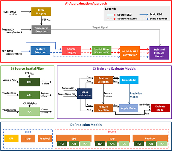
Figure 1. (A) Approximation approach, including the steps to extract the BOLD signal from the FEPN network and the EEG processing steps needed for deriving the 12 tested models. (B) For the source-based models, different spatial filtering strategies were explored: 1) ROI: average source signal across the target region, the FEPN; 2) AAL: average source signal across parcels defined according to the anatomical labelling atlas (AAL [39];); and 3) ICA: the IC time-courses from a spatial ICA step applied to the source-reconstructed EEG data or features. (C) Training and evaluation of the models based on a 6-fold cross-validation framework. (D) A total of 12 models were derived: the EFP (in yellow) represents the only method currently used in the literature. The scalp methods include also the iEFP and FeatPool, while the source methods include the EEG, iEFP and the FeatPool, each one obtained from the ROI, AAL and ICA spatial filtering strategies.
Download figure:
Standard image High-resolution image2.6.1. EEG features extracted
Seven EEG features were considered to build the proposed pool of features (the FeatPool model), three of which extracted from the time-frequency domain; the remaining four were focused on exploring the nonlinear characteristics of the EEG signal. The latter were motivated by previous studies showing their usefulness on several applications, including the characterization of mental imagery processes similar to the ones conveyed by the participants during the NF runs of the present study [16, 40, 41]. Furthermore, a nonlinear relationship between neuronal oscillatory activity and hemodynamic changes in the brain has been recently identified during rest [42], showing a strong association between fluctuations of the BOLD signal and both spectral features and nonlinear dynamic properties of spontaneous EEG. Our study is the first one, to the best of our knowledge, which sought BOLD correlated activity of nonlinear EEG dynamics during a task.
All features were estimated for each frequency band (by previously band-passing the EEG signal across the respective band), and for each 2-second EEG segment. For the time-frequency domain, we used the power, frequency peak (f-peak) and the Teager energy. The power was computed by squaring the signal and averaging its values. The f-peak was obtained by extracting the maximum values of the frequency spectrum. The Teager energy operator calculates the instantaneous energy of the signal x using

where ![$\Psi \left[ . \right]$](https://content.cld.iop.org/journals/1741-2552/17/4/046007/revision2/jneab9a98ieqn1.gif) denotes the Teager operator [43]; the resulting values were then averaged. This operator is sensitive to variations in both amplitude and frequency of the original signal x.
denotes the Teager operator [43]; the resulting values were then averaged. This operator is sensitive to variations in both amplitude and frequency of the original signal x.
For the nonlinear domain, we transformed the EEG signal into its phase-space, which represents an approximation of its chaotic dynamics. As shown by Takens [44], the phase-space captures the relevant properties of the state space representation of the system, such as the Lyaponov exponents and the Kolmogorov-Sinai Entropy. Every state of the system can be represented by a point in the multidimensional phase space, and the time evolution of the system creates a trajectory in this space [45]. We used the time delay embedding method to approximate the phase-space of the EEG. Given a time series x, the corresponding vector X in phase-space at time
  is given by
where  is the time delay,
  is the dimension of approximated space and
  is the number of points (states) in the phase-space. We approximated a 2- and 3-dimensional phase-space associated to the EEG data, and the time delay was considered to be the mean of the first local minimum from the autocorrelation of the signal (lag r) [46]. The phase-space trajectories represent system dynamics that tend to incorporate a bounded subspace referred to as an attractor. To characterize the attractor and the corresponding dynamics of the system, measures can be taken to estimate its complexity and stability. To estimate complexity, we computed the correlation dimension (CorrDim) of the trajectories, which is the most common approach. For the stability, we used the largest Lyapunov exponent (Lyap) and two entropy measures—approximate entropy (ApEn) and sample entropy (SampEn)—that quantify the chaos of the attractor [47].
The correlation dimension is a measure of the space fractal dimensionality. Correlation sum is defined as the sum of the fraction of pairs of points in the phase-space whose distance is smaller than r (the previously defined lag). If this number of points is sufficiently large, the ratio between the logarithm of the correlation sum and the logarithm of the time delay is an accurate estimate of the correlation dimension [48].
The largest Lyapunov exponent characterizes the rate of separation of infinitesimally close trajectories of the signal in phase space, yielding a measure of the degree of the instability of the system [48]. Mathematically, two trajectories in the phase space with initial separation of  , diverge at a rate given by

where  is the local Lyapunov exponent (local exponential rate of expansion). The maximum Lyapunov exponent corresponds to the mean exponential rate of divergence, characterizing the trajectory's instability.
The approximate (ApEn) and sample (SampEn) entropy quantify the regularity and predictability of signals throughout time. The ApEn is a descriptor of the changing complexity in the embedded space. The SampEn is a variation of the ApEn method which does not depend on the length of the signal and showing usually shows better relative consistency [49]. Since ApEn and SampEn present different values for the same characteristic of the signal, we considered both metrics in our analysis.
2.6.2. Addressing the hemodynamic delay of the BOLD signal
In order to tackle the hemodynamic delay of the BOLD signal relative to the EEG signal, the previously proposed EFP method incorporates in the regression problem not only the original spectral power predictors, but also their time-delayed versions up to 12 s [12]. Thus, the approximation model associated with this method is described by:
with y the BOLD signal to approximate at time t,  the k-th EEG feature, considering m features and n delays; and f the approximation function.
However, the most common approach to take into account this delay in conventional EEG-informed fMRI studies is to convolve the EEG time-course of interest with the canonical HRF [11]. Therefore, the EEG feature time courses xk were then convolved with the canonical HRF:

yielding the model

Because of the known variability of the HRF across subjects and sessions [50] and even brain regions [51], the EEG features were also convolved with HRF functions peaking at different latencies (3, 3.5, 4, 4.5, 5, 5.5, 6, 6.5, 7, 8, 10 and 12 s):

thus resulting in the final model:
with l the number of latencies (in this case, twelve, matching the number of delays considered in the EFP method). These three approaches (delays, canonical HRF and multiple HRFs) were tested on the EEG spectral power features used in the EFP method. Because the multiple HRF convolution approach yielded the highest approximation accuracy (apACC, see Results section), it was then considered for the new models proposed here.
2.6.3. Approximation models
We considered as baseline model the EFP, adapted from Meir-Hasson's work [12], consisting of the spectral power feature from seven frequency bands and their time-delayed versions, extracted from the scalp EEG signal. In this case, a total of 840 predictors (7 frequency bands × 12 delays × 10 channels) comprise the model used in the EFP method. We then tested the same method using the multiple HRF convolution approach. We named this method improved EFP (iEFPscalp), which also consists of 840 predictors (7 frequency bands × 12 latencies × 10 channels). Still at the scalp level, we tested the effect of using all the seven features (FeatPoolscalp), rather than the spectral power alone, also using the multiple HRF convolution approach. This results in the most complex model, with a total of 5880 predictors (7 features × 7 frequency bands × 12 latencies × 10 channels).
At the source level, three different spatial filtering strategies were explored. First, the region of interest (ROI; the FEPN) mapped in the localizer run was used for extracting the average source signals. Next, in order to consider whole-brain source activations, rather than those from the FEPN alone, the brain was parceled into 90 non-overlapping regions according to the AAL atlas [39] (see supplementary table S1), from which the source signals were averaged. Finally, a spatial ICA step [52] was first performed (using the FSL's tool MELODIC [53]) on the source signals from the localizer run (SSloc), and then the source signals from the remaining NF runs (SSNF) were projected onto the spatial IC maps of the localizer run (SMloc) in order to obtain the IC time-courses of SSNF (TCNF) in the localizer IC space:
In this way, the time-consuming ICA step only needs to be performed for the first functional run, while the concept of targeting with NF brain activity identified in the localizer run is preserved.
For each spatial filtering strategy (ROI, AAL and ICA), different source signals were considered, namely those computed from the source mapping of the EEG signal ( ), and of the features extracted for the iEFP (
 ) and the FeatPool (
 ) models. The source signals from the 3 [spatial filtering] × 3 [source mapping] = 9 source-based models were then submitted to the multiple HRF convolution approach, yielding a total of R× 12 (latencies), R× 84 (7 frequency bands × 12 latencies) and R× 588 (7 features × 7 frequency bands × 12 latencies) predictors, for the
  ,
,  and
and  models, respectively. R denotes the number of regions or ICs involved in the spatial filtering step: R= 1 for the ROI and R= 90 for the AAL; a variable number of ICs were computed across runs and subjects, the optimal number being estimated by MELODIC based on the eigenspectrum of the SSloc covariance matrix.
2.6.4. Approximation approach
The abovementioned models were then compared in terms of their approximation accuracy (apACC), defined as the Pearson correlation between the average BOLD signal across voxels in the FEPN (identified by the localizer run; section 2.4.2) and the approximated BOLD signal resulting from the regression procedure using each of the several compared models. In order to obtain estimations of the apACC values, the three NF runs were first concatenated (generating, for each subject, fMRI datasets of 900 volumes), and then split into training and test sets by a 6-fold cross validation scheme, having so the equivalent of half of a NF run in each test set. For each fold, the associated portion of the BOLD signal is approximated. After having the full signal approximated by the six folds, the apACC was computed by correlating the measured BOLD signal with the approximated one.
Given the high number of predictors in most models tested, the minimum redundancy maximum relevance (mRMR) method was used for feature selection, which ranks the features to include in the different models [54]. This way, the risk of overfitting is minimized [55]. In order to investigate the impact of model complexity in the approximation of the BOLD signal, we varied the number of predictors included in the models according to the mRMR. Specifically, models with 1, 2, 5, 10, 20, 50, 100, 150, 200 and 250 predictors were considered; more complex models were not tested since apACC reached a plateau in most cases. For models with a total predictor count below 250 ( : 12 predictors;
  : 84 predictors) the range of predictors considered was upper-bounded by that value. This way, we tested the
  model with 1, 2, 5 and 10 predictors, and the
  with 1, 2, 5, 10, 20 and 50 predictors.
For the regression step, random forests were used with bootstrap aggregation (bag) of an ensemble of decision trees (number of random predictors per split: number of predictors/3, minimum number of observations per leaf: 5), as implemented in the MALTAB R2019b's Statistics and Machine Learning toolbox fitrensemble function (method: Bag, number of learning cycles: 150). Random forests were selected for their capacity to deal with small sample sizes and large feature sets, outperforming competing machine learning algorithms in several studies [56, 57].
2.6.5. BOLD upsampling effect
The EFP method, as presented in [12], performs an upsampling of the BOLD signal by a factor of 8 (new sampling frequency of 4 Hz) using spline interpolation. We believe this induces strong linear relations on the target signal that will positively bias the apACC of the model. This was verified by investigating the impact of the upsampling step on the EFP model. Otherwise, all the results presented in the paper are conducted at the original BOLD sampling rate of 0.5 Hz.
2.7. Statistical analysis
In order to compare the performance of the models, we first determined the optimal number of predictors to be included in each model. For that we used the Akaike Information Criteria (AIC), simplified for regression model comparisons [58]:
using the original signal (y), the signal approximated by the model (y'), the number of samples in y (n; with i = 1..n), and the number of predictors used by the model (K). The AIC is then computed for each number of predictors considered (up to 250, see above); the optimal number of predictors is determined by minimizing the AIC. Then, the apACC values of the resulting models were submitted to a one-way repeated measures analysis of variance (ANOVA) to assess differences in their means. From that, we conducted post-hoc pairwise comparisons between each pair of models, correcting for multiple comparisons using the Tukey-Kramer method.
For assessing the statistical significance of the BOLD approximation achieved by the best model ( ), we ran permutation tests whereby the BOLD signal to be approximated was first permuted in time, followed by the training of
  with the permuted signal and the computation of its apACC [59, 60]; this procedure was repeated for 500 permutations of the BOLD signal. The statistical significance value was then defined as the percentage of permutations that achieved higher apACC when compared with that of
  when trained with the true BOLD signal.
Additionally, correlation maps from the EFP method (baseline model), FeatPoolscalp and  were also computed in order to verify the brain regions related to the approximated BOLD signal of the EFP and FeatPool models (scalp and source). For that purpose, we used the approximated signals separately as regressors of interest in a GLM analysis of the pre-processed fMRI data using FILM [28]. Voxels exhibiting significant correlations were identified by cluster thresholding (voxel Z > 2.7, cluster p < 0.007). Group activation maps were then obtained using the FSL's Local Analysis of Mixed Effects (FLAME) [61]. With this analysis, it was possible to assess if the brain regions associated with the approximated BOLD signal match those involved in the FEPN.
Afterwards, we investigated the contributions of each feature, frequency band and HRF latency to the approximation of the BOLD signal. We built histograms for each feature, frequency band and HRF latency used by the FeatPool models. We also analyzed the relative contribution of each channel and AAL region to the FeatPoolscalp and  models, respectively. Understanding which frequency bands and features contribute the most for the BOLD approximation provides insights into the electrophysiological mechanisms underlying the BOLD signal measured at the FEPN.
3. Results
3.1. BOLD upsampling effect
The effect of the upsampling step of the BOLD signal on the EFP model is presented in Figure 2. While it increases the number of time points by a factor of 8, strong, yet false, linear relationships between neighboring BOLD samples are introduced by the spline interpolation, which in turn inflates the accuracy in an artificial manner, verifiable both in the average apACC (across folds and participants) and the standard error of the mean. In fact, although the EFP model reached an average apACC of 90% when considering the upsampled BOLD signal, at the original sampling rate, such accuracy did not go beyond 20%.

Figure 2. Comparison of the original EFP model with and without upsampling the BOLD signal, considering different number of predictors included. The center of each bar represents the mean apACC of all participants between the approximated signal and the BOLD activity of the FEPN, and the error bars represent the standard error of the mean. The apACC reached a plateau at approximately 50 predictors.
Download figure:
Standard image High-resolution image3.2. Comparison of the approaches addressing the BOLD hemodynamic delay
Regarding the approaches considered for dealing with the hemodynamic delay of the BOLD signal, Figure 3 shows the effects of using the original approach applied to the EFP (delays), the approach used in conventional EEG-fMRI studies (convolution with the canonical HRF), and the new proposed method considering the convolution with multiple HRFs peaking at different latencies. Because the latter largely outperformed the other two (apACC of 48%, vs. 40% and 20% for the canonical HRF and delays approaches, respectively), only the convolution with multiple HRFs was considered for the remaining models; in particular, the new version of the EFP model using this approach was termed improved EFP (iEFP).
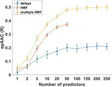
Figure 3. Comparison of the apACC achieved using the EFP method by the three approaches tested to tackle the hemodynamic delay. The HRF method only shows up to 50 predictors because it contains only the power for 7 frequency bands from 10 electrodes (70 predictors), while the other two have the different delays or the convolution with multiple HRFs, thus increasing the number of predictors (in these cases, 840). Points represent the group mean apACC values (computed between the original BOLD signal and the one approximated by the respective model) and the bars the standard error of the mean.
Download figure:
Standard image High-resolution image3.3. Comparison of the approximation accuracy of the models
The analysis for the optimal number of predictors based on the AIC for each model is presented in table 1. For most models, higher apACC values were consistently obtained by increasing the number of predictors (up to 250) included in them; however, we also observed that increasing the number of predictors from 150 to 200, or from 200 to 250, yielded a non-significant increase in the respective apACC values in most cases.
Table 1. Optimal number of predictors selected, for each model, based on the AIC values, and their respective mean and standard deviation of the AIC and apACC values.
| Model | # predictors | AIC (±std) × 103 | apACC (±std) |
|---|---|---|---|
| EFPscalp | 50 | −15.8 (±0.8) | 0.20 (±0.08) |
| iEFPscalp | 50 | −17.0 (±0.7) | 0.48 (±0.04) |
| FeatPoolscalp | 100 | −17.0 (±0.8) | 0.52 (±0.05) |
 |
5 | −15.5 (±0.7) | 0.15 (±0.07) |
 |
20 | −16.6 (±0.8) | 0.38 (±0.05) |
 |
100 | −17.0 (±0.7) | 0.50 (±0.04) |
 |
50 | −16.8 (±0.8) | 0.42 (±0.04) |
 |
50 | −16.9 (±0.8) | 0.46 (±0.04) |
 |
50 | −16.9 (±0.8) | 0.46 (±0.05) |
 |
50 | −17.2 (±0.8) | 0.50 (±0.05) |
 |
50 | −17.4 (±0.8) | 0.53 (±0.04) |
 |
100 | −17.4 (±0.8) | 0.56 (±0.05) |
Considering for each model the number of predictors with minimum AIC, Figure 4 shows the apACC values achieved by each model and post-hoc pairwise comparisons between them. Comparing with the EFP, only the  model did not surpass its apACC; in contrast, all the BOLD approximations from the other proposed models obtained statistically significantly higher apACC values. At the scalp level, the FeatPoolscalp outperformed the iEFPscalp model, showing that the pool of features is able to capture additional task-specific brain processes that are not fully identified using only the EEG power. At the source level, the same pattern was observed, with the FeatPoolsource exhibiting better results than the iEFPsource (for ROI, AAL and ICA spatial filtering strategies). As expected, using the information from several brain regions parceled according to the AAL, rather than the FEPN alone, higher correlation values were obtained. Finally, the ICA method was able to achieve the highest apACC, surpassing all other models from either the scalp or source spaces.
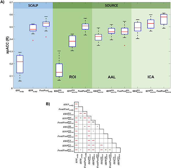
Figure 4. (A) Boxplot comparing the apACC values achieved by each model. (B) Significance matrix highlighting the pairwise statistical differences between the models (* p < 0.05, ** p < 0.01, *** p < 0.001, corrected for multiple comparisons by the Tukey-Kramer method).
Download figure:
Standard image High-resolution imageBased on the group correlation maps shown in Figure 5, it is possible to observe that by using both the FeatPoolscalp or the  models (the best models at the scalp and sensor levels, respectively), the brain regions associated with the approximated BOLD signal match those involved in the FEPN (mapped from the Localizer run at the group level), which is not observed when considering the EFPscalp model. Additionally, permutation tests on the best model
  further support its statistical significance, with the apACC values on all 500 permutations never surpassing the apACC achieved by the true model.
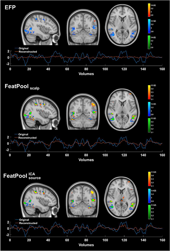
Figure 5. Group correlation maps (in red-yellow) for the EFPscalp model (top), the FeatPoolscalp model (middle; best at the scalp level) and the  model (bottom; overall best) (MNI coordinates: x = − 52, y = − 48, z = 6), superimposed on the group FEPN mapped from the localizer run (in blue-light blue); overlapping regions are highlighted in green. The FeatPool methods recover most of the FEPN, while the EFPscalp method fails to reconstruct even its main regions. Different z-score thresholds were considered for each model given their distinct statistical power. Below each group correlation map, the measured (in blue) and the approximated (in red) BOLD signals from the localizer run are shown, for a representative participant.
Download figure:
Standard image High-resolution image3.4. Importance of the features, frequency bands and HRF functions for the BOLD approximation
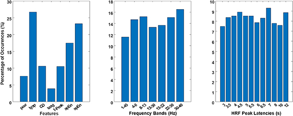
Considering the  as the best model to approximate the BOLD signal from the FEPN, we then investigated which features, frequency bands and HRF functions (among the top ranked predictors according to the mRMR feature selection method) contributed the most for the approximation (Figure 6). We verified a strong contribution from the largest Lyaponov exponent and the entropy features. For the frequency bands, the gamma band was the most used, followed by the high-beta, alpha and theta. Besides the largest contributions of HRF functions peaking at 7 and 12 s, the contribution of the remaining delays was evenly distributed, slightly prevailing, however, peak latencies around 4.5 s (i.e. close to the canonical HRF). We performed a similar analysis for the
  and
and  models; the results are shown in Supplementary Figure S1. Consistently with the
  model, a strong contribution of features from the nonlinear domain, as well as the theta and alpha frequency bands can be observed.
Figure 6. Histograms for the features, frequency bands and HRF functions used in the  model.
Download figure:
Standard image High-resolution image
4. Discussion
In this study, we systematically investigated the extent at which the BOLD-fMRI signal recorded from the facial expression processing network (FEPN) during a neurofeedback task could be approximated from the simultaneously recorded EEG signal. We proposed novel EEG features for approximating the BOLD signal, as well as new approaches to tackle its hemodynamic delay. Using random forests for the regression, we compared our novel contributions with the EFP (the only currently used model in the literature) and found that combining our newly proposed features with the convolution of multiple HRFs peaking at different latencies, mapped at the source space and projected onto the ICs computed for the localizer run, yielded the best model ( ), achieving an approximation accuracy (apACC) of 56%. This represented an improvement in 36 percentage points relative to direct comparison with the currently available EFP model.
4.1. Novel EEG features and the frequency bands considered
The FeatPool models outperformed the iEFP ones (improved EFP; models comprising only power spectral features convolved with multiple HRFs), showing that only spectral characteristics of the EEG are not sufficient to fully capture the BOLD signal variance at the target region, since the exploration of other characteristics of the EEG signal increased the apACC values substantially. Furthermore, we verified that the nonlinear features strongly contributed to the BOLD approximation for the FeatPool models, especially the ones that characterize the stability of the phase-space attractors, namely the largest Lyaponov exponent and the sample and approximate entropy. Importantly, other studies have already shown the pivotal role of nonlinear aspects of the EEG signal in mental imagery tasks, especially in the brain-computer interfaces domain [62–65]. The relationship between the BOLD signal and nonlinear EEG characteristics has already been established during rest [42]. Here we show that those nonlinear features can also be related to the BOLD signal of task-specific networks, particularly the FEPN. Importantly, nonlinear features are robust to the presence of noise [66], with their discriminative values remaining unaffected at high noise levels [67].
We also verified a strong contribution of features extracted from the theta band and high-beta/gamma bands, which is in line with our previous study where nonlinear features in the theta band discriminated the mental imagery of facial expressions processes of autism spectrum disorder patients from controls [16]. Importantly, EEG power over the theta and beta bands has been shown to exhibit significant correlations with the BOLD signal in the prefrontal cortex during memory tasks [68, 69]. Nevertheless, given the known sensitivity of spectral power fluctuations from the theta band to motion artifacts in simultaneous EEG-fMRI studies [70, 71], we quantified the amount of variance of predictors derived from the theta band explained by fMRI-derived motion parameters [72–74], and verified that it was only 6% on average across predictors, runs and subjects. This, coupled with our results reinforcing the relationship between EEG power over the theta band and facial emotion processing [16, 75, 76], based on the observed strong contribution of this frequency band for the approximation of the BOLD signal at the FEPN, rules out the possibility of the observed theta band fluctuations being a consequence of movement artifacts.
The fact that our data were acquired during a validated task involving well-defined brain areas comprising the facial expression processing network (FEPN) [15], coupled with the ability of the proposed  model to recover the FEPN (and therefore a clear neural correlate) according to our correlation maps, suggests that the approximated BOLD signal by
  reflects the neural processing of interest, rather than noise (based on the robustness of nonlinear features to noise and low explained variance of theta-based regressors by fMRI-derived motion parameters) or overfitting (according to the results of the permutation tests), and thus supporting the functional meaning of our results.
A successful transfer of fMRI NF interventions intrinsically relies on the ability of the chosen NF protocol to modulate the targeted signal (in our case, the BOLD activity at FEPN), which can be hampered by the presence of BOLD fluctuations of non-neuronal origin. Here, we were not able to remove respiratory-related fluctuations, which have been recently shown to confound the feedback signal (connectivity estimates) provided to the participants, with a global signal regression step being suggested as a possible solution [77]. However, global signal regression is a highly controversial step because it induces whole-brain spurious correlations, and thus may have adverse effects on the analyses [78]. Coupling these considerations with the fact that the NF protocol used in this study has been shown to successfully modulate the brain activity at FEPN in our previous studies [15, 79], we believe that respiratory fluctuations did not critically impact our analyses. This is further supported by the correlation maps of the best models (FeatPool), because otherwise approximations of a respiratory-contaminated BOLD signal at the FEPN would preclude its accurate recovering.
4.2. Tackling the BOLD hemodynamic delay
The EFPscalp method does not include any a priori knowledge on the BOLD hemodynamic response, letting the regression procedure weight each delay according to its contribution to the final approximation. This is different from conventional EEG-correlated fMRI studies, whereby the predictors are typically convolved with the canonical HRF (with a fixed delay of 5 s), thus including the expected behavior of the BOLD response [11]. We verified that, for the same number of predictors, convolving the predictors with the canonical HRF outperformed the 'delays' approach used in the EFP model in terms of the approximation accuracy of the BOLD signal. In [12], a similar comparison is also presented; however, the 'delays' approach surprisingly outperforms the canonical HRF convolution in this case. These contradictory results may result from unfairly comparing models with different complexities, with the original EFP model comprising twelve (the number of delays) times more predictors than those used when considering the convolution with the canonical HRF.
Motivated by the known variability of the HRF [50, 51], Sato and colleagues [80] followed an approach similar to the 'delays' approach used in the EFP model to estimate the transfer function between the EEG and the BOLD signal measured at the visual cortex. Despite their promising results, only two pilot subjects were considered, which limits the generalization of the results. Nonetheless, the morphology of the estimated transfer functions varied significantly across participants and experiments, thus supporting the convolution of the proposed EEG features with multiple HRF functions peaking at different latencies. For the same number of predictors, this approach outperformed the 'delays' and convolution with the canonical HRF approaches, possibly because it not only incorporates the hemodynamic response behavior in the predictor time course, but also addresses the variability of the HRF function, which has already been observed across subjects, sessions and brain regions [50, 51].
Some insights can also be derived from the analysis of the higher ranked (according to the mRMR) HRF latencies used in the best model (the  ). While the canonical HRF and its smaller variations were the most frequently used in the regression analysis, the
  model also exploited HRF functions deviating from the canonical HRF. The relevance of such larger latency peaks has also been previously reported [81, 82], but never in the context of task-specific studies. Our results are in agreement with those of Feige and colleagues [82] who observed that, depending on the EEG spectral band or network/region of interest, the lag between the EEG phenomenon and the corresponding deconvolved BOLD signal representative of different resting-state networks varied from 0 to 10.5 s. This highlights the importance of exploring different HRF modulation approaches, especially when integrating different imaging modalities.
4.3. Scalp- versus source-based approximation models
The source-based models also provided different results: the  model, which comprises the average source time-course across the FEPN from the direct mapping of the EEG signal, did not surpass the original EFPscalp model. Despite the expected gain in sensitivity by considering the more informative 3D space of the source, rather than the 2D space of the scalp, volume conduction induces redundancy between adjacent brain regions, which may compromise this source model extracted from such small regions as the FEPN [83]. However, when considering the source model comprising the parcel-averaged source time-courses (
 ) or the ICA-based time-courses (
 , the apACC improves significantly, suggesting that despite the volume conduction problem, whole-brain source activations convey crucial information for the approximation of the BOLD signal at the FEPN. Consistently, the source models considering the ICA outperformed the equivalent ROI and AAL versions. The fact that ICA is able to identify the underlying networks of the sources signals associated with the localizer may be crucial for separating task-specific fluctuations from the remaining ones, since the AAL brain parcellation method is blind to task specificities.
Exploring EEG source activations over time itself represents a new contribution to this field, as only a number of studies have explored this approach and its relationship with the BOLD signal in the context of disease (epilepsy) or resting-state. Specifically, the average source time-course across an epilepsy-related ROI has been shown to improve the epileptic network mapping with simultaneous EEG-fMRI, when compared with the typically used unitary regressors to model the BOLD signal [32]. More recently, resting-state networks, which are typically observed in fMRI, were shown to be also present on continuous EEG source data [33, 34, 84, 85]. Importantly, we have recently shown the feasibility of using continuous EEG source imaging (cESI) to study task-induced fluctuations on simultaneous EEG-fMRI data [79]; in the present study, we used cESI to derive source time courses as predictors in the approximation of the BOLD signal. The cESI processing steps conducted here were motivated by previous studies investigating the impact of such steps on detecting RSNs from resting-state cESI data, and particularly showing that eLORETA yielded the most accurate RSNs when compared to minimum norm estimates (MNE) and linearly constrained minimum variance (LCMV) [33]. The choice of the inverse model is known to influence the spatial extent and resolution of the solutions; however, the optimal inverse model is application-dependent, with a recent study suggesting that despite the lower spatial resolution of eLORETA solutions when compared to MNE and LCMV, eLORETA is less prone to the detection of false positives, and overall recommended unless a clear hypothesis can be formulated [86]. Although the cESI pipeline chosen here was not optimized for the purpose of approximating the BOLD signal, it was shown that source localization results are the most stable across ESI pipelines, when compared with estimations of functional and effective connectivity, suggesting that our cESI data may be robust to different cESI processing steps [87].
The fact that the FeatPool models clearly surpassed the improved EFP models suggests that the combination of different kinds of features (linear and nonlinear) was pivotal for the BOLD signal approximation. As shown in [88], the isolated use of features is unable to perform a direct mapping of the BOLD modulation in the FEPN. Moreover, the convolution of the several features with different HRF functions critically improved the approximation of the BOLD signal of interest. We were able to clarify the isolated effects of the feature set and delay approach, and this dissociation should help future studies to target both domains (features and delays) of EEG-fMRI transfer functions.
4.4. Impact on the transfer and dissemination of fMRI NF interventions to EEG setups
According to our results, it is clear that the EFP model presents multiple flaws. From a technical point of view, the upsampling step in its original implementation unrealistically allows the model to achieve very high apACC values, which are drastically reduced if the original sampling rate is considered. Additionally, in the original paper [12], the EFP model was developed for the purpose of approximating the BOLD signal measured at the amygdala; however, the reported correlation map does not show co-activations in areas known to interact with the amygdala, namely the prefrontal or limbic regions [89, 90]. Moreover, based on our correlation maps, we also observed that the EFP was unable to recover our region of interest (the FEPN), in contrast with the proposed  model. Such observations raise the hypothesis that the current EFP approximations may be partially derived from overfitting, evidencing the relevance of this study.
Building on their previous work [12], Meir-Hasson and colleagues created a generalized EFP model using the data from a subset of participants from which the most accurate approximation of the BOLD signal was achieved [14]. Although modest, the approximation accuracies were found to be statistically significant, and therefore this generalized EFP model has been since applied in several clinical trials of high impact [91–93]. The low accuracy achieved by a universal model is expectable due to the intrinsic inter-subject variability that both fMRI [94, 95] and EEG [96, 97] techniques present. Hence, we followed the more conservative approach of developing subject-specific models. These are particularly relevant for multi-session interventions [6, 98], whereby subject-specific models can be derived from one or a few sessions of concurrent EEG-fMRI, which are then used offline for personalized NF training. This approach relies on the intra-subject stability of the signals across sessions, which is more likely to be achieved than stability across subjects [99, 100]. Future studies should address this aspect for the proposed models. Nevertheless, given the significant increase in the approximation accuracy of the BOLD signal achieved by our proposed  model, we expect that the efficacy of these NF interventions would substantially improve with the adoption of our method, with direct impact on the prognostic of the patients being submitted to them. Naturally, this hypothesis could only be confirmed by effectively comparing the outcomes of NF interventions determined according to the EFP and
  models. Importantly, there is no insight in the literature regarding how accurate the approximation of the BOLD signal should be to ensure a feasible transfer.
The feasibility of building a model in real-time depends on the complexity of the features to be included in the model, and also on the technological capacity of extracting those features within reasonable computational times as to provide the feedback signal to the participant without a significant delay. Despite the complexity of some of the features included in the proposed  model, our pipeline takes around 250 ms to extract all the features in every channel on a PC of standard computational power. Thus, a new feedback sample can then be presented much faster than the feedback timing used in this study (2 s, matching the TR of the fMRI runs). More importantly, such timings are also reasonable when transferring this NF protocol to EEG setups [101, 102]. Interestingly, the
  model achieved a similar accuracy to that of
  , being however more computationally efficient as it does not require the extraction of features. This aspect may be crucial in studies where a limited computational power is available, or whenever a high rate of feedback delivery to the participants is needed [103]. The FeatPoolscalp model may be useful for EEG setups with limited scalp coverage, since we showed that a comparable accuracy to that of the best model can be achieved using features derived from only 10 electrodes.
5. Conclusion
In this study, we found that exploring nonlinear EEG features as the largest Lyapunov exponent or the sample and approximate entropies extracted from different frequency bands was crucial for more accurately approximate the BOLD signal measured at the facial expression processing network. Furthermore, by projecting such features into the source space, spatially filtering them by independent component analysis (ICA) and convolving them with multiple HRF functions peaking at different latencies, yielded substantial improvements on the BOLD signal approximation from the EEG data. Our proposed BOLD approximation model may therefore positively impact the transfer of fMRI-based neurofeedback interventions to EEG setups, and more importantly, their dissemination and efficacy in modulating the activity of the desired brain areas. Future studies should address how these models generalize across subjects and sessions and possibly explore new EEG features to further improve the approximation of the BOLD signal by the EEG alone, and also assess the level of accuracy needed for a successful transfer of fMRI-NF interventions to EEG setups.
Acknowledgments
Supported by The European Commission, under the Health Cooperation Work Programme of the 7th Framework Programme, with the Grant Agreement BRAINTRAIN—Taking imaging into the therapeutic domain: Self-regulation of brain systems for mental disorders [FP7-HEALTH- 2013-INNOVATION-1–602186 20, 2013]; FLAD Life Sciences, 2016; FTC—Portuguese national funding agency for science, research, and technology UID/4950/2017—COMPETE, CONECT-BCI | POCI-01-0145-FEDER-030852—PTDC/PSI-GER/30852/2017, PAC MEDPERSYST POCI-01-0145-FEDER-016428, SFRH/BD/77044/2011.