

Abstract
We have developed spectral models describing the electroluminescence spectra of AlGaInP and InGaN light-emitting diodes (LEDs) consisting of the Maxwell–Boltzmann distribution and the effective joint density of states. One spectrum at a known temperature for one LED specimen is needed for calibrating the model parameters of each LED type. Then, the model can be used for determining the junction temperature optically from the spectral measurement, because the junction temperature is one of the free parameters. We validated the models using, in total, 53 spectra of three red AlGaInP LED specimens and 72 spectra of three blue InGaN LED specimens measured at various current levels and temperatures between 303 K and 398 K. For all the spectra of red LEDs, the standard deviation between the modelled and measured junction temperatures was only 2.4 K. InGaN LEDs have a more complex effective joint density of states. For the blue LEDs, the corresponding standard deviation was 11.2 K, but it decreased to 3.5 K when each LED specimen was calibrated separately. The method of determining junction temperature was further tested on white InGaN LEDs with luminophore coating and LED lamps. The average standard deviation was 8 K for white InGaN LED types. We have six years of ageing data available for a set of LED lamps and we estimated the junction temperatures of these lamps with respect to their ageing times. It was found that the LEDs operating at higher junction temperatures were frequently more damaged.
Export citation and abstract BibTeX RIS

Original content from this work may be used under the terms of the Creative Commons Attribution 3.0 licence. Any further distribution of this work must maintain attribution to the author(s) and the title of the work, journal citation and DOI.
1. Introduction
Since the revolutionary invention of blue light-emitting diodes (LEDs) in the early 1990s, quickly followed by white LEDs with luminophore coating by the Nobel Laureates Isamu Akasaki, Hiroshi Amano and Shuji Nakamura [1], the lighting industry has been striving towards LED-based light sources, including light bulbs and street lights. Recently, it has been demonstrated that LED technology can also be used in optical metrology because, for example, photometric calibrations could be carried out in the future using LEDs rather than incandescent lamps as light sources [2–4].
LED lamps have longer lifetimes (>20 000 h) than conventional incandescent lamps (1000 h–2000 h) and fluorescent lamps (>10 000 h) [5]. Generally, there are several factors affecting the lifetime of the LED products, e.g. the quality and operating conditions of driver electronics [6], decreasing luminous flux due to the degradation of luminophore coating, and darkening of the diffuse bulb, which is usually made of polymers or glass. In addition, high junction temperature and high current density of LED chips have been considered to be factors limiting their lifetime [7]. Usually, the LED junction is the main source of heat in an LED product. Depending on the thermal management of the LED lamp, also components, such as thermally fragile electrolytic capacitors in the driver electronics, may experience extreme heat, leading to an early failure of the LED lamp [8].
In the case of consumer lighting products, especially AC-operated LED lamps with built-in electronics, the only non-invasive way to estimate the possible magnitude and change in the junction temperatures of LED components is usually via the emission spectrum of the product. Some methods to obtain junction temperatures spectrally have been developed. The slope method by Vaitonis et al [9] and the peak shift method by Chen and Narendran [10] model a narrow region of the spectrum. Some other optical methods, such as the double gaussian method by Ohno [11] and the semi-empirical method by Keppens et al [12], model the whole spectrum and they fit well to the experimental spectra. Obtaining the actual junction temperature of LED lamps is difficult with these methods because they need multiple spectra to be measured at known junction temperatures or have multiple steps in their calibration routine.
In this paper, we present improved spectral models for LEDs based on the Maxwell–Boltzmann statistics for the high-energy side of the spectrum, and on the effective joint density of states (DOS) of electrons and holes for the low-energy side. Our spectral model can be calibrated from a single spectrum at a known temperature. The models, when fitted, can be used to derive the junction temperatures of the LEDs and to predict their spectra at various junction temperatures. Separate DOS functions have been derived for red aluminium gallium indium phosphide (AlGaInP) and blue indium gallium nitride (InGaN) LEDs. The DOS model for the blue InGaN LEDs is also applied to white LEDs with luminophore coating and to LED lamps utilizing such LEDs. We also introduce a method by which the required reference spectrum at a known temperature can be conveniently obtained. For lamps, the spectral transmittance of the polymer or glass bulb needs to be taken into account.
In the next section, we introduce the light sources studied. These include a selection of LED lamps, as well as blue, white and red LEDs disassembled from these lamps. The spectral models for red AlGaInP and blue InGaN LEDs are introduced in section 3. The additional factors that need to be taken into account when applying the spectral models to white LEDs are also discussed in this section. A selection of the lamps has undergone a natural ageing test for a period of 50 000 h. In section 4, we use the model to estimate the junction temperatures of the LEDs within these lamps throughout their lifetimes, and compare the results with the noted ageing of the lamps. Finally, conclusions are drawn in section 5.
2. Experimental data
2.1. Description of LEDs
The lamp types studied with their key parameters are presented in table 1. At the beginning of the work, several new specimens of each five lamp type were chosen for different types of tests to study their ageing mechanisms. Some lamps were studied as they are, some were disassembled to extract the individual LEDs used as building blocks of the lamps, and some underwent ageing tests of different types. From the lamps selected, the Osram PAR16, Classic A40 and Classic A60 utilized blue InGaN LEDs with luminophore coating. Osram Classic A80 contained red AlGaInP LEDs in addition to InGaN LEDs with luminophore coating. Philips Master LED consisted of LED printed circuit boards (PCBs) and a bulb with remote luminophore plates. The disassembled LED PCBs consisted of uncoated blue InGaN LEDs.
Table 1. Characteristics of four lamp specimens of five different LED lamp types studied in this work. Luminous flux, power consumption and correlated colour temperature (CCT) were measured for each lamp specimen at the beginning of the natural ageing. One extra lamp of each lamp type was disassembled and characterized for the driving electronics and the number of LED components. The LEDs in lamps PAR16 and CL A40 are driven by pulse-width-modulated (PWM) current. Estimated lifetime in the last column has been specified by the manufacturers.
| Manufacturer | Type | Luminous flux/lm | Power/W | CCT/K | Number of LEDs | Current/mA | Lifetime/h |
|---|---|---|---|---|---|---|---|
| Philips | Master LED | 869.8 | 12.80 | 2683 | 18 | 205 (DC) | 25 000 |
| 850.0 | 12.78 | 2681 | |||||
| 823.6 | 12.74 | 2684 | |||||
| 836.5 | 12.54 | 2686 | |||||
| Osram | PAR16 | 252.3 | 4.47 | 6723 | 3 | 300–790 (PWM 38 kHz) | 35 000 |
| 242.0 | 4.24 | 6512 | |||||
| 250.2 | 4.41 | 6266 | |||||
| 259.3 | 4.25 | 6583 | |||||
| Osram | CL A40 | 377.2 | 7.86 | 3063 | 6 | 0–840 (PWM 41 kHz) | 25 000 |
| 365.4 | 7.87 | 3080 | |||||
| 370.3 | 7.84 | 3047 | |||||
| 376.9 | 7.79 | 3034 | |||||
| Osram | CL A60 | 732.5 | 12.53 | 3071 | 9 | 380 (DC) | 25 000 |
| 756.4 | 12.80 | 3073 | |||||
| 700.0 | 12.61 | 3089 | |||||
| 746.3 | 12.53 | 3062 | |||||
| Osram | CL A80 | 878.2 | 13.34 | 2802 | 12 | 370 (DC) | 25 000 |
| 876.6 | 13.34 | 2885 | |||||
| 890.1 | 13.48 | 2808 | |||||
| 906.3 | 13.73 | 2859 |
The LED PCBs of all lamps disassembled were further equipped with conducting wires and studied in oil baths to derive the relationships between the forward voltage, junction temperature and operating current [13, 14]. The LEDs were driven by current pulses with a pulse length of 1.9 ms repeated every 10 s. The self-heating effect due to the pulses [15, 16] was not corrected from the forward voltage measurements, but afterwards the effect was studied with the result that the junction temperatures may be underestimated by 1 K to 3 K with low current levels of a few 100 mA. The self-heating becomes more pronounced at higher current levels. The LED spectra were measured at known temperatures by applying knowledge of the forward voltage over the LED. The final dataset contains the electroluminescence spectra of three LED specimens of each LED type (one red, one blue and four white types) at various known temperatures and electrical current levels.
Figure 1(a) presents the spectra of all lamp types tested. Although all the lamps are mainly based on blue LEDs with luminophore coating, the spectra deviate significantly from each other. The cool white spectrum of Osram PAR16 is obtained with yellow luminophore and Osram Classic A80 consists of similar yellow luminophore and red AlGaInP LEDs [18, 19]. The rest of the bulb types produce warm white light by mixing green, yellow and red luminophores in different ratios.
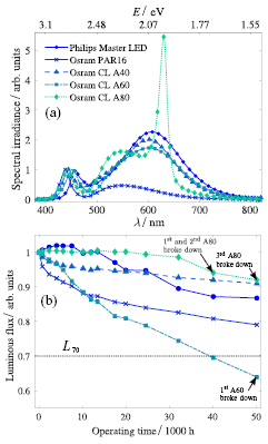
Figure 1. Emission spectra of five commercial LED lamp types studied (a) and their average relative luminous flux degradation as a function of ageing time (b). The dotted line represents the lifetime standard L70 [17] of the LED lamps, according to which the lamp meets its lifetime when the luminous flux drops below 70% of the initial luminous flux. The lamp specimens that broke down, such that they did not produce light, were excluded from the results in (b).
Download figure:
Standard image High-resolution imageWe have six years of ageing data available for a set of LED lamps [5]. Four lamps of each type were aged under laboratory conditions and monitored periodically for luminous flux, luminous efficacy, relative spectral radiant flux and correlated colour temperature (CCT). Such long-term monitoring requires a reliable realization of the absolute scale of luminous flux, and thus all the luminous flux measurements made in monitoring the lamps were carried out using an integrating sphere facility with an expanded uncertainty of 0.9% [5, 20]. All spectral data measured for the ageing test were corrected for the spectral responsivity of the integrating sphere photometer, as well as for the spectral self-absorption of the lamps. Figure 1(b) shows the average relative luminous flux as a function of time for the different types of lamps.
2.2. Methods to obtain LED spectra at known temperatures
The spectral models introduced later in this work need one spectrum at a known temperature to obtain material parameters for the DOS before the model can be used to derive junction temperature from measured spectra.
The forward voltage method, developed by Xi and Schubert [13] and JEDEC [14, 21], is one of the most accurate methods of calibrating individual LEDs for their junction temperature against the forward voltage of the LED. The forward voltage method is based on the old industry standard MIL-STD-750D [22], more specifically method 3101.3 that was adapted from the publication by Siegal [23]. The LEDs are submerged in a temperature-controlled oil bath and each LED is driven by short current pulses with simultaneous forward voltage measurement. As each LED component has its individual forward voltage properties, such calibration needs to be carried out separately for each LED. After the calibration, the LED spectrum at a known temperature can be measured by driving the LED with direct current corresponding to the amplitude of the current pulses during calibration and by varying the heatsink temperature until the forward voltage reaches the desired value.
The method by Zong and Ohno [24] applies the forward voltage method [13]. Instead of an oil bath, the LED is mounted on a heatsink, which can be set at temperatures between 10 °C and 100 °C. When no current is flowing through the LED, its junction and the heatsink are at the same temperature. The LED is driven by an electrical pulse and the forward voltage is measured simultaneously over the LED junction. Then, the LED is operated with a direct current that matches the amplitude of the pulse used in the calibration. The heatsink is cooled or heated until the forward voltage reaches the calibrated voltage. The junction temperature is now known and the spectrum can be measured. Later, self-heating of a few kelvins was observed even with short current pulses, and thus extrapolation of the rising temperature to the start of the pulse [15] was added to the method and documented to CIE 225:2017 [16].
We have studied the possibility of deriving an LED spectrum at room temperature, without the need for any synchronous measurements that could potentially be applied to LED lamps with a dimming option. An LED is driven by a pulse-width-modulated electrical current and the modulation ratio is changed. The electrical power causing excess heat that raises the junction temperature, reduces as the modulation ratio drops. For linear systems, the junction temperature waveform for any modulation ratio can be obtained from measurement of the step response [25]. The spectrum at ambient temperature can be constructed by extrapolating the relative changes in the spectral irradiance at each wavelength to the duty cycle of 0% according to figure 2. Duty cycles above 10% were used in order to reduce the effect of thermal transients close to the rising edge of the current pulse. One way to estimate whether these distortions are dominant is to check which normalized spectra intersect at the temperature-invariant energy value introduced in [26]. Broadened spectra affected by transients do not pass through the intersection point of other spectra and are excluded from the analysis.

Figure 2. Electroluminescence spectra of a red AlGaInP LED (a) and the blue peak of a white InGaN LED (b), driven by 1 kHz rectangular current (0 mA–200 mA). Coloured dotted curves depict spectra measured with the various duty cycles and the black solid curve depicts the spectrum extrapolated to the room temperature of 298 K.
Download figure:
Standard image High-resolution image3. Spectral models for LEDs
The electroluminescence spectrum  of an LED is defined by the DOS
  of electrons and holes multiplied by the Fermi–Dirac distribution as

where  is the photon energy with the reduced Planck constant
  and angular frequency ω. Parameters Ec and Ev are the conduction band and valence band energies. Fermi–Dirac distributions determine the thermally induced occupation probabilities of the electrons in the conduction band and the holes in the valence band [27, 28] as
where kB is the Boltzmann constant, Tj is the junction temperature, and Efn and Efp are quasi-Fermi levels with subscripts fn and fp that refer to negative and positive charges.
We approximate the Fermi–Dirac distributions with Maxwell–Boltzmann statistics because we do not know the exact quasi-Fermi energies of the electrons and holes in the active region with biased conditions [29]. With the Maxwell–Boltzmann approximation, the spectral model becomes
where  is the bandgap energy, which depends on the junction temperature according to the Varshni formula [30] as
with the material-specific parameter values α and β. For ternary semiconductor alloys like InxGa1−xN, the effective bandgap becomes [31]
where x is the mixing ratio and  is the bowing parameter.
  and
and  are obtained from equation (5) with the Varshni parameters listed in table 2.
Table 2. Varshni parameters of GaN and InN by Vurgaftman et al [31].
| Semiconductor |  /eV /eV |
α/meV K−1 | β/K |
|---|---|---|---|
| GaN | 3.507 | 0.909 | 830 |
| InN | 1.994 | 0.245 | 624 |
The Maxwell–Boltzmann approximation is valid at low current densities and at high current densities for carriers above Efn and below Efp [27, 28, 32]. Using this simplification, the effective DOS of an LED can be calibrated by fitting the spectral model of equation (4) with the effective DOS model multiplied by the Maxwell–Boltzmann distribution to the measured spectrum at the known junction temperature [27, 28, 33]. The effective DOS can be further modelled with equations introduced in sections 3.1 and 3.2 depending on the materials of the active layer.
3.1. Red AlGaInP LED
In our earlier studies [33], we modelled the spectra of the red AlGaInP quantum-well LEDs at various junction temperatures. These LEDs are similar to those in Osram Classic A80 lamps. In [33], the spectrum of an LED at a temperature of 303 K was divided by the corresponding Maxwell–Boltzmann distribution, and the obtained DOS was modelled as two exponentially broadened step functions:
where A1 and A2 are the step heights,  and
and  are the broadening parameters, and
  is the split-off energy of the sub-bands. For AlGaInP LEDs, the splitting of the valence band arises from the spin–orbit interactions [31]. According to our experiments, parameters
  ,
,  meV,
meV,  meV and
  meV are common for a specific LED type at varied junction temperatures and operating currents. Thus, they only need to be obtained once for each LED type. The absolute step heights and parameters Eg,
  and
and  depend on Tj and operating current and thus need to be fitted for each normalized spectrum measured. Alternatively, as the bandgap energy
  is a function of Tj, it can be modelled using the Varshni formula with the mixing ratios x and y of a quaternary (AlyGa1−y)xIn1−xP alloy [31] as free parameters. Both ways produce the same results.
Experiments by Katahara and Hillhouse [34] and Wu et al [35] have shown that an exponentially broadened step function also describes the effective DOS of gallium arsenide (GaAs) LEDs and indium nitride (InN) thin films.
Junction temperatures obtained by modeling were compared with calibrated Tj obtained by the forward voltage method over the temperature range 303 K–398 K at current levels of 200 mA, 300 mA and 370 mA. The standard deviation between the modelled and measured junction temperatures was about 2.4 K (0.7%) and the maximum difference was 8.5 K [33]. When our method was compared with the slope method [9] and the peak shift method [10], it gave the most accurate junction temperatures while being able to model both sides of the spectra.
3.2. Blue InGaN LED
The temperature dependence of the electroluminescence spectrum emitted by a blue InGaN LED obtained from a Philips Master LED lamp is shown in figure 3. The spectra were measured using the setup and methods described in more detail in [33]. The modelled spectra (black solid lines) were fitted to measured spectra (coloured dotted lines) by the relative least-squares fitting method [36, 37]. Figure 4 presents the effective DOS obtained by fitting the spectral model to the measured spectrum with the Maxwell–Boltzmann distribution at the known temperature. Similar effective DOS shapes have been measured by, e.g. Nakamura [38], O'Donnell et al [39], Wang et al [27] and Lock et al [40]. As can be seen, the DOS does not follow an exponentially broadened step function as was the case for AlGaInP and GaAs LEDs. Instead, we have developed another DOS model,
where A1 is the step height;  breaks the symmetry of the sigmoid function with the broadening parameters
  and
and  . Parameters that need to be calibrated using the reference spectrum at the known temperature are
  ,
,  and
and  . The step height A1, bandgap energy
  and the additional broadening parameter
  change with changing Tj. The effective mixing ratio x in
  of equation (6) was also set as a temperature-independent free fitting parameter so that the spectral model with the DOS parameters calibrated could be used to model the spectrum of other LED specimens of the same type. The spectral range of ±0.22 eV around the energy corresponding to the spectral irradiance peak was modelled.
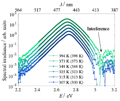
Figure 3. Spectra of InGaN LED #1 measured (coloured dotted lines) at 205 mA and various junction temperatures, and the fitted model (black solid lines). Legends state the modelled junction temperature for each spectrum and the corresponding reference junction temperature in parentheses. The normalized spectrum measured at 348 K was used to calibrate the model parameters. All spectra are shifted in the vertical direction for clarity.
Download figure:
Standard image High-resolution image
Figure 4. Density of states of the InGaN LED #1 measured at 205 mA (coloured dotted lines) and the model fits (black solid lines) on a linear scale (a) and logarithmic scale (b). Each density of states was normalised to the energy of 2.9 eV. The model parameters used for fitting were calibrated at 348 K.
Download figure:
Standard image High-resolution imageIdeally, the DOS of a quantum-well LED should form a step function. There are multiple mechanisms that may distort the InGaN DOS from this ideal form. The spectral peak emission of blue InGaN LEDs can be varied from 3.4 eV to 2.0 eV by increasing the indium content during the manufacturing process, until the collapse of the crystal structure [41]. The dislocations of the InGaN lattice arising from the lattice mismatch of the layers may reach ∼109 cm−2 [42], and thus the DOS is broadened due to the variations in the local indium content and the spatial thickness in the quantum-well layer [29, 43], whereas the AlGaInP and GaAs LEDs can be grown with high crystal quality with dislocations less than ∼103 cm−2 [42]. The deep localized states of the local indium-rich environment form excitons near the bound states [43, 44]. Such excitons are hydrogen-like systems and they have localized energies. At low temperatures with low carrier densities, they can be seen as additional peaks at the edges of each energy state contributing to the DOS [44]. Actually, the spin–orbit and crystal-field splitting of the valence band states can be determined from the exciton peaks present in reflectance and photoluminescence data measured at extremely low temperatures, e.g. 2 K [45].
What we see in the measured InGaN DOS in figure 4 is the rising edge of the lowest energy state [46], distorted by potential fluctuations of the lowest radiative states. A metallic p-contact acting as a mirror is sometimes used to enhance the light emission from the LED chip, which causes interference. Figure 3 shows the interference [47, 48] at 3.05 eV for the emission spectrum of Luxeon flip-chip blue LEDs [49] of Philips Master LED lamps.
The model in equations (4) and (8) was tested on three blue InGaN LEDs from Philips Master LED lamps operated at six values of Tj between 303 K and 398 K and four current levels I. The DOS parameters were calibrated against the normalized spectrum of LED #1 measured at  K and I = 205 mA. These model parameters were then used to derive junction temperatures of other spectra at various Tj and I, and also of spectra of the two other LED specimens of the same type. The junction temperatures derived are compared with the known reference temperatures presented in table 3. As can be seen, the model varies slightly. Differences change as a function of Tj and I, but mostly for different LED specimens. The standard deviation between the three samples over all the temperatures and current levels of table 3 is 11.2 K. The varying temperature introduces a standard deviation of 1.8 K and the varying current a standard deviation of 2.1 K. The results indicate that the model parameters vary among specimens and to a smaller extent as a function of Tj and I. The sample-to-sample variation can be explained to a large extent by variations in the material substrate and their effects on the DOS. The mixing ratios x converge to sample-specific values of
  for LED #1,
  for LED #2 and
  for LED #3. If each LED specimen is calibrated separately using one spectrum at a known temperature, the overall standard deviation between the modelled and measured junction temperatures decreases from 11.2 K to 3.5 K.
Table 3. Differences  between the modelled and the reference junction temperatures of InGaN blue LEDs extracted from the Philips Master LED lamp. Calibration of the DOS parameters was carried out by fitting the spectral model in equation (4) with the DOS model of equation (8) to an experimental spectrum of LED #1 measured at the known junction temperature of 348 K and a current of 205 mA. Other spectra (also for LEDs #2 and #3) were modelled using these calibrated parameters so that the junction temperature was one of the fitting parameters.
| LED #1 | LED #2 | LED #3 | ||||||||||
|---|---|---|---|---|---|---|---|---|---|---|---|---|
| I/mA | 100 | 150 | 205 | 250 | 100 | 150 | 205 | 250 | 100 | 150 | 205 | 250 |
| Tj/K |  /K /K |
 /K /K |
 /K /K |
|||||||||
| 303 | −0.7 | 2.3 | 3.4 | 4.1 | 9.9 | 15.2 | 18.4 | 19.1 | −15.4 | −12.0 | −10.3 | −13.8 |
| 313 | −0.5 | 1.4 | 2.0 | 3.8 | 7.8 | 12.6 | 16.9 | 18.7 | −17.3 | −13.7 | −11.2 | −10.5 |
| 323 | −2.2 | 0.5 | 1.7 | 3.5 | 7.8 | 12.2 | 14.2 | 16.8 | −15.1 | −12.5 | −11.9 | −11.4 |
| 348 | −2.0 | 0.1 | −0.3 | 0.6 | 8.8 | 11.0 | 13.4 | 15.2 | −14.1 | −11.6 | −10.5 | −11.7 |
| 373 | −1.7 | −0.4 | −0.4 | 0.0 | 11.0 | 13.8 | 14.1 | 15.1 | −15.2 | −13.2 | −12.7 | −11.7 |
| 398 | −4.3 | −3.3 | −3.9 | −2.8 | 9.1 | 11.3 | 13.1 | 13.0 | −16.8 | −15.9 | −15.7 | −14.1 |
 /K /K |
−1.9 | 0.1 | 0.4 | 1.5 | 9.1 | 12.7 | 15.0 | 16.3 | −15.7 | −13.1 | −12.0 | −12.2 |
3.3. White InGaN LEDs
White LED spectra are spectrally more complex than blue LED spectra due to the photoluminescence of the luminophore coating. Modelling the photoluminescence would require knowing the absorption, excitation and emission spectra of each luminophore type used in the final mixture, and the thickness of the luminophore layer [50]. As the lamps studied in this work are of commercial type, we do not have access to such data, and thus we have to use more practical methods to account for the photoluminescence. The broadening parameters  and
and  of the effective DOS model in equation (8) can account for distortion by the photoluminescence. In addition, since the electroluminescence spectra of red LEDs can be modelled using equation (7), we separated their spectra from the white spectra of Osram Classic A80 according to figure 5.

Figure 5. Relative spectra of red AlGaInP and blue InGaN LEDs extracted from the white spectrum of an Osram Classic A80 lamp. The red and blue LED emission spectra are influenced by the photoluminescence (PL) of the luminophore coating in the blue LEDs.
Download figure:
Standard image High-resolution imageThe spectral model developed for blue InGaN LEDs, validated using the blue LEDs extracted from Philips Master LED lamps, was tested on three white InGaN LEDs from Osram PAR16, Osram Classic A60 and Osram Classic A80 lamps. Osram Classic A40 was left out of the analysis because the blue peak and photoluminescence overlapped considerably. The LEDs were operated at their nominal currents as stated in table 1, at values of Tj between 303 K and 423 K. Three specimens of each LED type were considered. The effective DOS for each LED type was determined by determining DOS separately for the three LED specimens and averaging the model parameters. Spectra at other temperatures were then analyzed to derive optical junction temperatures that were compared with the known reference temperatures. The results are presented in table 4. Results are given as the averages of the LED specimens with standard deviations. On average, the standard deviation among the three white LED types is 8 K. Table 5 presents the average model parameters obtained for the different LED types.
Table 4. Average differences  between the modelled and the reference junction temperatures of three InGaN LED specimens of each lamp type with their standard deviations. The spectra were measured with direct currents of 205 mA for Master LED, 790 mA for PAR16, 380 mA for CL A60, and 370 mA for CL A80. The spectral ranges fitted are between
  eV for Master LED, and between
  eV and
  eV for PAR16, CL A60 and CL A80. We could not measure all spectra of LED specimens of Master LED, CL A60 and CL A80 due to limitations in cooling and heating their junction.
| Lamp type | Master LED | PAR16 | CL A60 | CL A80 |
|---|---|---|---|---|
| Tj/K |  /K /K |
 /K /K |
 /K /K |
 /K /K |
| 303 |  |
 |
 |
— |
| 313 |  |
 |
 |
— |
| 323 |  |
 |
 |
— |
| 348 |  |
 |
 |
 |
| 373 |  |
 |
 |
 |
| 398 |  |
 |
 |
 |
| 423 | — |  |
— |  |
 /K /K |
 |
 |
 |
 |
Table 5. Average model parameters describing the effective DOS for each LED type, derived from the relative electroluminescent spectra measured at 348 K.
| Parameters | Master LED | PAR16 | CL A60 | CL A80 |
|---|---|---|---|---|
 /meV /meV |
18.63 | 19.20 | 21.07 | 20.43 |
 /meV /meV |
69.13 | 50.63 | 53.17 | 55.67 |
 /meV /meV |
117.5 | 105.5 | 142.1 | 129.9 |
4. Estimated junction temperatures of LED lamps
The methods presented are also to some extent applicable to lamps, i.e. by measuring the lamp spectrum, an estimate for the average Tj of the LEDs within the lamp can be derived by following the steps in figure 6. Because of our extensive studies of the LED specimens of the lamps described in sections 3.2 and 3.3, it was not necessary to apply steps 1–3. Instead, we tested the scheme starting from step 4 for all of the lamps except for the Osram Classic A40. For the DOS, we used the data for LEDs in table 5. In addition to these parameters, we also accounted for the bulb transmittance of the lamps.
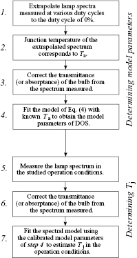
Figure 6. Steps to estimate the junction temperature Tj of an LED lamp. Parameter Ta is the ambient room temperature. Steps 1 and 2 are described in section 2.2.
Download figure:
Standard image High-resolution imageThe bulb materials of LED-based light sources are usually made of translucent polymers or glass. The cut-on wavelength depends on the bulb type as shown in figure 7. The transmittances were determined from the relative spectra of the lamps measured in  geometry using a 1.65 m integrating sphere spectroradiometer [20], including spectral self-absorption measurements of the lamps with and without the bulbs attached. The Philips Master LED has remote luminophore plates, whose effective spectral absorptance spectrum was determined from the ratio of the relative spectra measured with and without the remote plates. When modeling the junction temperature optically from the LED lamp, the transmittance or absorptance of the bulb has to be first corrected from the spectrum.

Figure 7. Effective bulb transmittances of Osram PAR16, CL A40, CL A60 and CL A80 lamps and effective absorptance of the remote luminophore bulb in the Philips Master LED lamp.
Download figure:
Standard image High-resolution imageUsually, an LED lamp contains multiple LED components, which may have slightly different optical characteristics, e.g. for their peak energy. This makes the sum spectrum measured appear broader than the spectrum of a single LED, which overestimates the junction temperature obtained. We studied this effect by deriving temperatures from a sum of three LED spectra, and the individual spectra, and comparing the results. The differences between the junction temperature determined from the sum spectrum and the average junction temperature obtained for the spectra of three LED components, using the average model parameters stated in table 5, were 6.9 K for Philips Master LED, 9.8 K for Osram PAR16, 1.2 K for Osram Classic A60 and 0.4 K for Osram Classic A80. The small differences in the case of Osram Classic A60 and A80 are explained by the uniformity of the LED specimens.
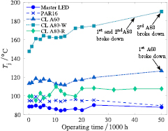
The average junction temperatures estimated for each LED lamp type are plotted in figure 8 as a function of their operating time. We do not know the real junction temperatures of the LEDs within the lamps, which complicates validation of the model. Results for LEDs given in table 4 indicate that their junction temperatures might have an average standard uncertainty of approximately 9 K because of the deviation of LED specimens. In addition, determining the junction temperature from the sum spectrum of LEDs may cause a systematic increase in the apparent junction temperature. The average standard uncertainty assigned to this effect is approximately 3 K. The bulb transmittance may also vary between lamp specimens. Overall, the expanded uncertainty of the optically derived junction temperature is 19 K (5%), excluding the effect of the bulb. The standard deviation of the junction temperatures obtained from different lamp specimens was between 6 K and 10 K, depending on the lamp type.
Figure 8. Average junction temperatures estimated for each LED lamp type. CL A80-W and CL A80-R refer to white LEDs and red LEDs inside the CL A80 lamp.
Download figure:
Standard image High-resolution image
Although the obtained junction temperatures have large uncertainties, they may be useful in comparing lamp types with each other, or in studying the changes of temperatures as we have done in figure 8. When we compare the junction temperatures of the lamps with the noted changes in luminous flux shown in figure 1(b), we do not see a clear correlation between junction temperature and change of luminous flux. Osram Classic A80, which according to the analysis has the highest junction temperature, degrades the slowest.
It is interesting to note that the driving electronics of A80 lamps started to break after approximately 40 000 h. The lamps were disassembled to study the condition of the LEDs. In the Osram Classic A80 lamp, all the six white and six red LEDs are connected in series, and all the LEDs are driven with the same direct current of 370 mA. Only 50% of the 24 white LED components produced light at 1 mA when they were driven by external current, 29% produced light at 10 mA, and 21% produced no light at 10 mA. In contrast, all the 24 Osram Classic A80 red LEDs worked fine and produced light at 1 mA. This indicates that the higher junction temperature breaks the LEDs because, according to the analysis, the junction temperatures of the white LEDs are significantly higher than those of the red LEDs.
The driving electronics of one of the Osram Classic A60 lamps broke after the final round of luminous flux measurements. According to the analysis, the junction temperature in this lamp is the second highest. Osram Classic A60 is also the only lamp that during the experiment met the end of its lifetime L70 [17] at around 40 000 h. The reason for the degradation of the luminous flux was darkening of the luminophore coating.
5. Conclusions
We have modelled the electroluminescence spectra of LEDs to derive their junction temperatures. The spectral models are based on the Maxwell–Boltzmann distribution and effective DOS derived from one spectrum at a known temperature. The spectrum at a known temperature may be obtained, for example, by using the forward voltage method or by driving the LED at varied duty cycles and extrapolating the results to zero duty cycle, corresponding to room temperature. This method could be used for determining the temperature characteristics of LED lamps by introducing a dimming option based on pulse-width modulation.
The spectral models work well for red AlGaInP LEDs, where the standard deviation between the modelled and known reference junction temperatures was 2.4 K over three LED specimens at the temperature range of 303 K–398 K and current levels of 200 mA–370 mA. For blue InGaN LEDs, the corresponding standard deviation was 11.2 K over the same temperature range with current levels of 100 mA–250 mA. Possible causes of the increased standard deviation in the case of blue LEDs include deviations in the reference junction temperatures and variability of the LED specimens. By calibrating each LED specimen separately, the standard deviation decreased to 3.5 K. The effective DOS appears to be slightly different for each LED specimen, possibly due to the manufacturing process, which limits the accuracy of the model compared with red LEDs. The model for blue LEDs was also to some extent applicable to white InGaN LEDs. The average standard deviation between the modelled and known reference junction temperatures was 8 K for three white LED types.
The method also gives average junction temperatures for the LEDs within an LED lamp, and it was used to analyze the junction temperatures of four lamp types undergoing natural ageing tests for 50 000 h. We could not validate these temperature determinations in the same way as the measurements of individual LEDs, because we had no access to the real temperatures of the LEDs within the lamps. We estimate the expanded uncertainty of the junction temperatures obtained to be 19 K (5%), mostly dominated by the variation of the LED specimens. There was no clear trend between junction temperature and the noted degradation in luminous flux. However, it appears that the lamps have started to break, beginning with the lamps with the highest junction temperatures.
In the future, determination of the optical junction temperature using the spectral models developed could be applied with imaging optics to other LED-based devices.
Acknowledgments
This work has been supported by the European Metrology Research Programme (EMRP) within the joint research project ENG05 'Metrology for Solid State Lighting'. The EMRP is jointly funded by the EMRP participating countries within EURAMET and the European Union. The authors thank Timo Dönsberg for building the voltage-to-current converter used in the pulsed measurements of the LEDs. György Andor is acknowledged for calibrating the LED components by the forward voltage method. AV would also like to acknowledge the funded position of Aalto ELEC doctoral school.