

Abstract
We present a tutorial on the determination of the physical conditions and chemical abundances in gaseous nebulae. We also include a brief review of recent results on the study of gaseous nebulae, their relevance for the study of stellar evolution, galactic chemical evolution, and the evolution of the universe. One of the most important problems in abundance determinations is the existence of a discrepancy between the abundances determined with collisionally excited lines and those determined by recombination lines: this is called abundance discrepancy factor (ADF) problem, and we review results related to it. Finally, we discuss the possible reasons for the large t2 values observed in gaseous nebulae.
Export citation and abstract BibTeX RIS

Original content from this work may be used under the terms of the Creative Commons Attribution 3.0 licence. Any further distribution of this work must maintain attribution to the author(s) and the title of the work, journal citation and DOI.
1. Introduction
There are two main types of gaseous nebulae that we will discuss in this review: H ii regions and planetary nebulae (PNe). Precise models of individual nebulae permit us to determine accurate abundances, which allow us to test models of stellar evolution, galactic chemical evolution, and the evolution of the universe as a whole.
H ii regions are sites where star formation is occurring. Therefore, H ii regions provide us with the initial abundances from which stars are made at present; abundances are paramount to test models of the chemical evolution of galaxies. For spiral galaxies they provide us with radial abundance gradients of heavy elements relative to hydrogen that have to be explained by models of galactic chemical evolution (Berg et al. 2013; Sánchez et al. 2014; Bresolin & Kennicutt 2015; Esteban et al. 2015; Magrini et al. 2016; Arellano-Córdova et al. 2016). Irregular galaxies that have a high fraction of their mass in the form of gas where almost no heavy elements are present, permit us to determine the primordial abundance of helium and hydrogen due to Big Bang nucleosynthesis (Ferland et al. 2010; Izotov et al. 2014; Aver et al. 2015; Peimbert et al. 2016).
PNe are produced by intermediate-mass stars, those in the 0.8 M⊙ to 8 M⊙ range, while they transit from the red giant stage to the white dwarf stage. The study of these nebulae show that intermediate-mass stars are responsible for most of the nitrogen, about half the carbon, and a non-negligible fraction of oxygen and helium present in the universe (e.g., Karakas & Lattanzio 2014). These stars also produce an important fraction of the slow neutron process elements, like rubidium, strontium, yttrium, zirconium, cesium, barium, lanthanum, and praseodymium. Big Bang nucleosynthesis created all of the hydrogen and deuterium; most of the helium; and a fraction of the lithium. Massive stars, those with more than 8 M⊙, produce most of the remaining elements, including the fast neutron process elements as well as a fraction of the helium, carbon, nitrogen, and oxygen abundances (e.g., Pagel 2009).
The classical textbook on the study of gaseous nebulae and active galactic nuclei is Osterbrock & Ferland (2006). This book discusses in depth the physical processes in PNe and H ii regions. It also mentions previous books and many review papers that presented earlier ideas and results on these objects. Other texts that in the past were considered fundamental in the study of photoionized regions are Stromgren (1939, 1948), Seaton (1960), Osterbrock (1974, 1989), and Aller (1984).
Other relevant review articles and books related to the physical conditions of gaseous nebulae are Kwok (2000) on the origin and evolution of planetary nebulae, Ferland (2003) on quantitative spectroscopy of photoionized clouds; Dopita & Sutherland (2003) on the astrophysics of the ionized universe; Stasińska (2004) on cosmochemistry the melting pot of the elements; Pagel (2009) on nucleosynthesis and the chemical evolution of galaxies; and Stasińska et al. (2012) on oxygen in the universe.
In the last few years there have been four meetings dedicated only to planetary nebulae. Two of the symposia organized by the IAU (Manchado et al. 2012; Liu et al. 2017) and two conferences on asymmetric planetary nebulae (Zijlstra et al. 2011; Morisset et al. 2014). The IAU Planetary Nebula Working Group produced a review paper on the present and future of PNe and their central stars research and related subjects (Kwitter et al. 2014).
Pérez-Montero (2017) recently published a tutorial that deals specifically with the determination of chemical abundances of H ii regions through the so-called direct method.
In this paper, we present a combination of a tutorial and a review paper on recent results related to the study of H ii regions and PNe. Section 2 describes some basic physical processes present in gaseous nebulae. Section 3 describes the main methods used to determine the physical conditions in gaseous nebulae. Section 4 discusses methods to determine the total abundances of the elements in gaseous nebulae, with special emphasis on the determination of the ionization correction factors to take into account the ions that are not observed. Section 5 presents recent results derived from the study of galactic and extragalactic H ii regions. Section 6 presents recent results derived from planetary nebulae. Section 7 includes a general discussion on possible physical reasons of why the temperature inhomogeneities are considerably higher than those predicted by photoionization models of chemically homogeneous nebulae. Some final remarks are discussed in Section 8.
2. Brief Discussion of Physical Processes in Gaseous Nebulae
There are several processes occurring in the ionized gas of planetary nebulae and H ii regions. In this section we briefly explain some concepts (such as photoionization, recombination, heating, cooling, and emission line mechanisms) that are necessary to understand the subsequent sections. It is beyond the scope of this paper to describe all of them in detail, and we suggest that the reader review the books and papers mentioned above (in particular, the book by Osterbrock & Ferland 2006) to understand the physics involved in these objects.
2.1. Photoionization and Recombination Processes: Local Ionization Equilibrium
The basis of the study of photoionized regions is to assume an equilibrium between ionization and recombination. It has long been known that in equilibrium a photoionized region will have a large volume of ionized gas surrounded by a relatively narrow transition zone where the gas goes from being nearly completely ionized to nearly completely neutral (e.g., Stromgren 1939; Osterbrock & Ferland 2006).
Because approximately 90% of the atoms of the ISM are hydrogen, for a first approximation the equilibrium is studied for a gas made up entirely of hydrogen atoms. Locally one must study the equilibrium between recombination and ionization:

where ne, np,  , represent the electron, proton, and neutral hydrogen density,
  represents the recombination coefficient for hydrogen at a given temperature,
  the energy required to ionize hydrogen (13.6 eV),
  represents the local radiation, and aν the ionization cross section of a given photon. In photoionized regions,
  dominates over
  and the ionization fraction is nearly one for most of the volume.
Globally, one can estimate the maximum volume that can be ionized by a constant ionization source. The first thing to notice is that recombinations to the ground level will produce photons with energy greater that  , thus they can be considered an additional source of ionization; this source usually accounts for approximately 40% of the ionizating photons. One solution to avoid this problem is to ignore recombinations to the ground level (as the subsequent ionization will cancel out the recombination). The recombination rate to all levels but the ground level is usually referred to as
  . Because there will be a steady rate of recombinations, ionizing photons will be required to keep a volume of gas ionized; those photons will be exhausted when a volume of size
  is ionized, where rS (the Strömgren radius) can be estimated as

where  represents the rate of ionizing photons produced by the central star, and
  ) the total hydrogen density.
For nebulae with realistic chemical compositions, the ionization of helium needs to be modeled as well as those of heavier elements. In general, neither will affect much the results for hydrogen, as helium recombination will, in general, return hydrogen ionizing photons, and the abundance of heavy elements is very small. However, the degree of ionization of heavy elements cannot be neglected because it turns out to be very important for the temperature equilibrium.
2.2. Heating and Cooling: Local Thermal Equilibrium
The previous results cannot be properly determined without knowing the physical conditions of the gas of the nebula. While the density is generally considered to be given by the characteristics of the gas previous to the photoionization, the energetics of photoionized regions are dominated by photoionization, and the temperature strongly depends on the physics of photoionization. As such, in equilibrium the temperature of the gas comes from a balance of local cooling and heating processes.
Heating will come from photoionizing photons, and hydrogen photoionization will account for at least 90% of this heating. Helium photoionization will account for 10%, or less of the total heating, while photoionization of heavy elements will only produce trace amounts of heating. Additional heating can come from dust photo-heating, or from free–free absorption, but neither will dominate the energetics.
The heating due to photoionization will be due to the excess energy of photoionizing photons beyond the ionizing threshold of the different atoms and ions (13.6 eV for hydrogen); consequently, it will be proportional to the number of photoionizations and to the temperature of the photoionizing star. On the other hand, in equilibrium, the number of photoionizations is equal to the number of recombinations, which in turn is proportional to the density squared for most of the object.
Other possible sources of heating are cosmic rays and shock waves; these are traditionally considered to be unimportant, thus they are ignored. However, while the former is not expected to be important, the latter can locally contribute with an important fraction of the heating (see Section 7).
To balance the heating, one must consider the possible sources of cooling. The most obvious source that must be considered is recombination where the kinetic energy of the captured photon is removed from the gas. This is, however, not the most important source of cooling.
If one were to consider a gas made up entirely of hydrogen (or hydrogen and helium), recombination would indeed be the best way to remove energy from the nebula. In this scenario, the heating is proportional to the temperature of the star and the cooling is proportional to the temperature of the nebula, so balance will occur when the gas has a temperature similar to that of the star (in fact, when done carefully, the gas ends up being hotter than the ionizing star). This is not seen in nature. Ionizing stars of H ii regions have temperatures of  K, while H ii regions often have temperatures of
  K; central stars of PNe have temperatures of
  K, while PNe often have temperatures of
  K. The difference is due to the additional cooling produced by forbidden lines excited by collisions.
2.3. Emission-line Mechanisms
The spectra of ionized nebulae are characterized by a weak continuum and strong emission lines. Figure 1 shows some of the most conspicuous emission lines: [O ii] λ3727, λ3729, Hδ, Hγ, Hβ, [O iii] λ4363, λ4959, λ5007 in the blue part of the spectrum, and Hα, [N ii] λ6548, λ6583, He I λ6678, [S ii] λ6717, λ6731, He I λ7065, [Ar iii] λ7135 in the red part of the spectrum.

Figure 1. Blue and red spectra for region A of NGC 346 obtained at CTIO with the 4 m telescope and the R-C spectrograph. The figures have been taken from Peimbert et al. (2000). © AAS. Reproduced with permission.
Download figure:
Standard image High-resolution imageThese lines are produced when an atom (or ion) is de-excited after being excited by photons or by collisions between atoms or atoms and electrons. The weak continuum is due to bound-free, free–free, two photon emission, dust scattered light, and starlight for extragalactic H ii regions. The main mechanisms producing emission lines are recombination, collisional excitation, and photoexcitation. One particular line can be produced by several mechanisms, but usually one of them dominates the others. Most of the strongest lines in ionized nebulae are produced by collisional excitation.
Deeper spectra allow us to measure the considerable fainter recombination lines. Figures 2 and 3 show three published echelle spectra of the H ii regions M8 and M17, obtained by García-Rojas et al. (2007) and the PN NGC 5315 obtained by Peimbert et al. (2004). These portions of the spectra show several recombination lines (such as C ii, O ii, N ii, Ne ii, and N iii lines) together with some collisonally excited lines of [Fe iii] and [Ar iv]. The broad emission feature in the spectra of NGC 5315 is due to the Wolf-Rayet type central star.

Figure 2. Sections of the echelle spectra of the Galactic H ii regions M8 and M17 obtained with the high-resolution spectrograph UVES at the Very Large Telescope. The figure has been taken from García-Rojas et al. (2007).
Download figure:
Standard image High-resolution image
Figure 3. Sections of the echelle spectrum of the Galactic PN NGC 5315 obtained with the high-resolution spectrograph UVES at the Very Large Telescope. The broad feature is due to the [WC4] Wolf-Rayet type central star. The figure has been taken from Peimbert et al. (2004). © AAS. Reproduced with permission.
Download figure:
Standard image High-resolution imageIn general, the intensity of an emission line,  , can be written as

where jλ is the emission coefficient,  is the density of the ion that emits the line,
  is the electron density, and
  is the emissivity. For example, the Hβ and [O iii] λ5007 intensity lines are given by


The emissivities of recombination lines (RLs) and collisionally excited lines (CELs) are discussed below.
2.3.1. Recombination Lines
RLs are produced when free electrons are captured by ions and descend from excited to lower levels emitting photons in the process. These lines are also known as permitted lines because they typically satisfy all the selection rules for an electric dipole transition. Most of the bright RLs in emission spectra are from hydrogen and helium. Metals such as carbon, nitrogen, and oxygen also produce RLs, but they are much weaker due to their lower abundances with respect to hydrogen and helium.
The emission coefficient of a recombination line,  , is given by

where  is the energy difference between the two levels and
  represents the effective recombination coefficient.
Some of the RLs that can be found in the spectra of ionized nebulae are H i lines (e.g., Hα at 6563 Å, Hβ at 4861 Å, Hγ at 4340 Å), He i lines (e.g., 5875 and 4471 Å), He ii lines (e.g., 4686 Å), O i lines (e.g., 8446 and 8447 Å), O ii lines (e.g., 4639, 4642, 4649 Å), O iii lines (e.g., 3265 Å), O iv lines (e.g., 4631 Å), C ii lines (e.g., 4267 Å), C iii lines (e.g., 4647 Å), C iv lines (e.g., 4657 Å), N ii lines (e.g., 4237 and 4242 Å), N iii lines (e.g., 4379 Å), N iv lines (e.g., 4606 Å), and Ne ii lines (e.g., 3694 Å).
The H i photons emitted by recombination may or may not escape. In an optically thin nebula, all the emitted photons will escape; this is known as Case A (Baker et al. 1938). On the other hand, in an optically thick nebula, all of the hydrogen Lyman photons will be absorbed; this is called Case B. The intermediate situations between these two extreme cases are explained below.
2.3.2. Collisionally Excited Lines
In contrast with hydrogen and helium, the energies of the first excited levels of some ions of heavy elements are within a few eV of the ground level, which makes it relatively easy to reach them through collisions with electrons. CELs are produced when the atoms excited through collisions decay via radiative transitions. Although the transition probability of these lines is low, the relatively low density of ionized nebulae, allows these transitions to occur. Some of these transitions, the ones produced in the optical range, are forbidden by the parity selection rule ( ), thus the emitted lines are often called forbidden lines. Others, called semi-forbidden lines, only violate the spin rule (
 ).
).
The emission coefficient of a collisionally excited line produced by a radiative transition from level k to level l is given by

where fk is the fraction of ions  in the upper level, k, and Akl is the spontaneous transition probability from level k to l. To compute the emissivity of a CEL, one needs to know the population of the upper level. It is necessary to solve the statistical equilibrium equations: the rate of population of a level by radiative and collisional processes is balanced with the rate of de-population by these processes:

where  and fk are the fraction of ions
  in the levels l and k, and qlk and qkl are the collisional de-excitation and excitation rates. The detailed expressions of qlk and qkl can be found in Osterbrock & Ferland (2006). To solve these equations, atomic data (collision strengths and radiative transitions) and an estimate of the physical conditions are necessary. Software such as PyNeb (Luridiana et al. 2015) and the iraf
1
package nebular provide a solution for the equations for a number of levels depending on the ion.
in the levels l and k, and qlk and qkl are the collisional de-excitation and excitation rates. The detailed expressions of qlk and qkl can be found in Osterbrock & Ferland (2006). To solve these equations, atomic data (collision strengths and radiative transitions) and an estimate of the physical conditions are necessary. Software such as PyNeb (Luridiana et al. 2015) and the iraf
1
package nebular provide a solution for the equations for a number of levels depending on the ion.
The CELs are one of the main cooling factors within ionized nebulae, so the presence of intense CELs depends on having available levels a few eV above the ground level. Because the temperature in photoionized nebulae is usually equivalent to about 1 eV, these differences are only available within the same ground-state electron configuration and therefore require the presence of a sub-shell with at least two electrons and two empty spaces to have the possibility of fine structure interaction between equivalent electrons to produce multiple levels within such configuration.
2.3.3. Fluorescence
Some permitted lines of some elements, such as oxygen, are brighter than expected by pure recombination because they are excited by starlight or by other nebular lines. The Bowen lines are one particular case of these lines; they are produced because there is a coincidence between the wavelengths of two lines. In this example, the O iii line at 303.80 Å and the He ii line at 303.78 Å. Some of the photons emitted by the He++ atoms are absorbed by the  atoms and then are re-emitted. Because the interpretation of fluorescence lines is complicated, they are preferably not used to derive physical or chemical parameters in nebulae; indeed, it is important to identify this type of lines in order to avoid them in the calculations.
Case C and Case D. From the early studies of photoionized regions, it was recognized that the hydrogen spectrum strongly depends on the optical depth of the Lyman lines as well as on the effect of the possible presence of fluorescence of the same lines. Baker et al. (1938) and Aller et al. (1939) defined Case A as the simplest possible case, where the nebula is optically thin; Case B, when the size of the nebula is such that the optical depth of the Lyman lines is so large that the fraction of such photons that escape is negligible; and Case C when the spectrum of an optically thin nebula is affected by fluorescence of hydrogen due to non ionizing continuum (Ferland 1999). Case B has been the most studied of these, as the physical conditions of most nebulae are closer to those of Case B than to those of cases A and C. Recently, it has been recognized that some objects are affected by both optical depth and fluorescence (Luridiana et al. 2009; Peimbert et al. 2016); this scenario is frequently called Case D.
In Case D, because the hydrogen transitions are optically thick, de-excitation occurs through higher series lines, in particular excitation to level n  produce transitions to
  , Balmer emissivities are systematically enhanced above case B predictions. Moreover, the He i lines are also enhanced by fluorescence. Case D produces small effects in the H i and He i lines, but they might be important in the determination of the primordial helium abundance.
Optical depth of levels other than the ground level. The first excited level of H decays too fast to be of any significance: heavy elements are not abundant enough to have very large optical depths; however, He0 is abundant enough and has a metastable level with a long enough half life to require special attention.
The effects on the helium abundance determination due to the optical depth of the 23S metastable level have been studied by Robbins (1968); Benjamin et al. (2002), and Aver et al. (2011).
3. Calculation of Physical Conditions and Ionic Abundances from Observations
Using the concepts described in Section 2 and the simple assumptions that the photoionized region is homogeneous in temperature, density, and chemical composition, it is possible to determine the physical conditions and chemical abundances of photoionized regions. To a first approximation, these three assumptions seem to be adequate (all the gas has a common origin, and photoionization models show that temperature should vary by only a few percent across most of each photoionized region). Careful study of the best observed objects, in particular the presence of abundance discrepancy factors (ADFs), show that at least one of those simplifications is not warranted.
In this section, we describe how, starting from observations of specific photoionized regions and atomic data sets, it is possible to determine the physical conditions (density and temperature) and the ionic chemical abundances. While presenting the determinations of ionic chemical abundances we will present two sets of chemical abundances: those derived from CELs and those derived from RLs; when both sets are available, RLs produce higher chemical abundances and their ratio is called the ADF.
3.1. Quality of the Available Spectra
Long-slit optical spectra have been widely used in the literature to derive the physical conditions and ionic abundances of ionized nebulae. There are spectra of several hundreds of Galactic and extragalactic PNe and H ii regions with resolutions better than ∼5 Å (see, for example, the compilations by Kwitter & Henry 2012; Maciel et al. 2017). These spectra allow the detection of nebular lines such as [O iii] λ4959, λ5007, [N ii] λ6548, λ6583, [S ii] λ6717, λ6731, as well as RLs from hydrogen, helium, and carbon (C ii λ4267). Deep long-slit spectra also allow the measurement of weaker lines such as the auroral lines [O iii] λ4363 and [N ii] λ5755. Some available long-slit spectrographs are LRIS at Keck I telescope, GMOS at Gemini telescope, FORS at Very Large Telescope (VLT), and OSIRIS at Gran Telescopio Canarias (GTC); many more spectrographs are available in smaller telescopes.
Echelle spectra provide a resolution better than 1 Å that allows us to separate and measure nearby lines, such as the mutiplet 1 of O ii at ∼4650, used to compute  abundances with RLs, whose lines can be contaminated with lines of N ii, N iii, [Fe iii]. The number of ionized nebulae with deep and high-resolution data in the literature is around 50 (see, e.g., the sample used by Delgado-Inglada et al. 2014). Some examples of echelle spectrographs are HIRES at Keck I telescope, MIKE at Magellan Clay telescope, and UVES at VLT; dozens of other echelle spectrographs are available in smaller telescopes, but one requires echelles at large telescopes to obtain deep and high-resolution spectra needed to study faint lines.
The use of Integral Field Unit (IFU) and multi-object spectrographs (MOS) allows the spatial study of ionized nebulae, often at the expense of a poorer spectral resolution. Several long-slit spectrographs are also MOS and some instruments may operate in both modes (MOS and IFU). A few examples of abundance studies based on IFU or MOS data can be found in Magrini & Gonçalves (2009), Stasińska et al. (2013), Kehrig et al. (2016), and Zinchenko et al. (2016). Some examples of MOS and IFU spectrographs are GMOS at Gemini telescope; FORS and VIMOS at VLT; and PMAS at the CAHA 3.5 m telescope. With the arrival of instruments such as MEGARA (Gil de Paz et al. 2016) in GTC, a high-resolution IFU and MO spectrograph, it will be possible to study ionized nebulae with a high spectral and spatial resolution.
3.2. Calibrations
Spectral emission lines allow the determination of physical conditions and ionic abundances in ionized nebulae. Before using spectroscopic data, one should remove the effect of the instrument and the atmosphere and perform some calibrations. This is called data reduction and it depends on the type of spectra (long-slit, echelle, multi-fiber, and integral field unit) and on the instrument and telescope. It is beyond the scope of this tutorial to explain in detail the whole process of data reduction, and we refer the reader to the web pages of the observatories (such as GTC2 , ESO3 , and GEMINI4 ) to find more information. One of the main packages used to reduce astronomical data is iraf 5 and there are many manuals available explaining how to use it.
In brief, the main steps in data reduction are bias and dark subtraction, cosmic rays removal, flat-field correction, wavelength, and flux calibration. The bias is the number of counts in the detector pixels for zero second exposures. The dark current is the number of counts in the pixels when no light is falling in the detector and it is caused by the movements of electrons in the electronics. Both signals need to be subtracted from all images. The flat-field image allows the correction of pixel-to-pixel variations due to differences in the sensitivity. Cosmic rays are high-energy particles that arrive into the detectors constantly and need to be removed, which is easy when there are various exposures of the same field. Wavelength calibration consists in the transformation of pixel scale into wavelength scale and it is done by using comparison spectra of lamps (such as Th-Ar, Ne lamps). And finally, flux calibration transforms the number of counts into intensities and for this, standard stars are required. Besides, one would like to trim the spectra, combine them into one final spectrum, then correct from: the Earth movement around the Sun, the interstellar reddening, and the earth atmospheric lines if possible.
The observation of the continuum and the emission lines of gaseous nebulae need to be corrected for interstellar extinction due to interstellar dust. We refer the reader to the discussion of this issue in Chapter 7 of Osterbrock & Ferland (2006).
3.3. Continuum Emission and Underlying Absorption in Nebular Spectra
The emission line spectra are superimposed on top of a weak continuum that has to be subtracted from the observations to recover the emission line intensities. The weak continuum is due to bound-free and free–free emission, two photon emission, dust scattered light, and starlight. For galactic objects it is possible to avoid the central star in PNe and the brightest stars in galactic H ii regions, but not for extragalactic H ii regions and PNe. Starlight will contain many permitted lines in absorption; of particular interest are the H i lines since they are used to calibrate most of the objects and can be significantly affected by underlying absorption. The errors produced by the underlying component can be minimized by studying objects with the highest equivalent width of Hβ in emission.
We consider that the best procedure to correct for underlying absorption in H ii regions is to use the models by González-Delgado et al. (1999, 2005). According to these models, for young objects the  (Hβ) is expected to be less than 2.5 Å, and at the same time the
  (Hβ) is expected to be more than ∼150; on the other hand, for older objects,
  (Hβ) is expected to be larger, while
  (Hβ) is expected to be smaller. The correction for underlying absorption for objects with
  (Hβ) > 150 Å is inversely proportional to
  (Hβ), while for objects with
  (Hβ) ≤ 150 Å the correction, and consequently the associated error, increases even faster due to the larger
  (Hβ) predicted by the models.
3.4. Atomic Data
The first step, when calculating the physical conditions and ionic abundances is to select the set of atomic data for your calculations. A different selection will translate into a different result. A compilation of some of the most used atomic data was provided by Mendoza (1983) and other recent compilations can be found on the CHIANTI6 and NIST7 web pages. Atomic physicists make a great effort providing us accurate atomic data, it is fair to give them the credit by citing the original papers where the atomic data are published.
Juan de Dios & Rodríguez (2017) recently discuss the impact of different sets of atomic data on the determination of the chemical abundances of O, N, S, Ne, Cl, and Ar.
The package PyNeb contains several sources of atomic data so that the user can choose their preferred ones. There is also a default set of atomic data recommended by the developers of PyNeb. The software iraf does not allow a simple change of the atomic data, but the adopted sources can be checked. The C17 version of the photoionization code cloudy (Ferland et al. 2013) allows for an easier treatment of the atomic data because the files have been moved to external databases.
3.5. Determination of Physical Conditions
The spectra of ionized nebulae show bright emission lines that allow us to determine the physical conditions of the gas: electron temperatures ( ) and densities (
 ).
).
The electron configurations with a complete sub-shell only have one specific configuration, thus one available level; ground configurations with a sub-shell with only one electron (as well as those lacking one electron to be complete), while theoretically able to have more than one configuration, have several configurations that are equivalent and thus have the same energy. For these three types of configurations, the first excited state requires at least one electron to move from one electronic shell to another. The amount of energy required for such transitions is (a) too high to be easily accessible via collisions and (b) lies in the ultraviolet. On the other hand, ions with ground-state electronic configurations of  ,
,  , and
, and  are easily observed (which have their first four excited levels with an energy
  , i.e., easily reachable via collisions and with some transitions in the optical range); the study of the intensities of these transitions has long been understood and many codes are available which can model the intensities of such lines as a function of temperature, density, and abundance. In principle, ions with electron configurations of the form
  (
( ) can also be studied in a similar manner, but ions with the required number of electrons are less abundant; also, because they have many more energy configurations available, software to model the behavior of such ions is less easy to obtain.
The p2, p3, and p4 ions have line ratios sensitive to the electron temperature. The number of electrons required for those configurations are exactly six, seven, eight, 14, 15, or 16; in principle, ions with 32, 33, and 34 electrons have the same configurations, but the most abundant of these would be Se++, which is five orders of magnitude less abundant than O+ and is too faint for its auroral lines to be seen. Some examples of observable ions are  ,
,  ,
,  , Ne++,
  ,
,  , Cl++, Ar++, and Ar+3.
The p3 ions have line ratios sensitive to the  . The numbers of electrons required for this configurations are exactly seven and 15; in principle, ions with 33 electrons have the same configuration, but the most abundant of these would be Se+, which is even less abundant than Se++ (although the relevant lines for traditional density determinations are nebular lines). Some examples of observable ions are:
  , Ne+3,
  , Cl++, and Ar+3.
The Grotrian diagrams for  ,
,  , and Ne++ obtained with PyNeb are presented in Figures 4–6.

Figure 4. Grotrian diagram for  from PyNeb (Luridiana et al. 2015)
Download figure:
Standard image High-resolution image
Figure 5. Grotrian diagram for  from PyNeb (Luridiana et al. 2015).
Download figure:
Standard image High-resolution image
Figure 6. Grotrian diagram for Ne++ from PyNeb (Luridiana et al. 2015).
Download figure:
Standard image High-resolution imageIn principle, we can also use di levels ( ) to calculate physical conditions, but the number of excited energy levels that need to be considered as well as the atomic physical parameters makes it impractical, and only a few of these ions have been studied (e.g., Fe++, Fe+3, and Ni++). Numerical packages used to study them are not widely distributed (PyNeb does contain these ions).
3.5.1. Electron Temperatures from CELs
The intensity ratios of some forbidden lines are highly sensitive to  , thus they are very useful in its calculation. The reason for that is that electrons with very different energy are needed to populate the different ionic levels of an ion through collisions.
For example, the excitation energy of level  , from which the [O iii] λ4363 line originates, is 5.35 eV, whereas the excitation energy of level
  , from which the [O iii] λ5007 line originates, is 2.51 eV (see Figure 4). Therefore, the ratio between these two lines tells us about the temperature of the plasma. We expect the intensity ratio of [O iii] λ4363/λ5007 to be higher in hotter nebulae.
In Chapter 5 of Osterbrock & Ferland (2006), one can find the analytical expressions for the intensity ratio [O iii] (I(4959) + I(5007))/I(4363) and other intensity ratios that are commonly used in the literature to estimate Te, such as [N ii] I(5755)/(I(6548) + I(6583)), [Ne iii] I(3343)/(I(3869) + I(3968)), and [S iii] I(6312)/(I(9532) + I(9069)).
The main disadvantage is that the auroral lines (such as [O iii] λ4363 and [N ii] λ5755) are weak, and if the observations are not deep enough, they are not detected. Alternative methods have been proposed to compute the chemical abundances when the  cannot be derived, such as the so-called strong line methods that will be discussed in Section 4.3.
3.5.2. Electron Temperatures from RLs
The intensity of a recombination line is approximately proportional to  . This approximation would result in ratios that are completely independent of the temperature, yet, when studied in detail, it is found that
  , where ϒ is the oscillator strength of each transition and has a weak temperature dependence which locally can be represented as
  where
where  . This approximation shows a small dependence on the temperature that can occasionally be exploited to determine the temperature using only RLs.
In reality, this is very difficult because the hydrogen lines have a nearly homogeneous dependence on T, and RLs of heavy elements are too weak to be used. The only remaining possibilities are temperatures determined from He, where the errors are at least ∼1000 K for the best observed objects (e.g., Peimbert et al. 2000, 2007; Izotov et al. 2007) or to try to combine one RL with a CEL (Peimbert & Peimbert 2013); in this last scenario, although the sensitivity of the ratios is similar to the sensitivity of nebular to auroral CEL ratios, the intensity of RLs is frequently smaller than that of auroral lines, thus the observational errors tend to be large.
3.5.3. Electron Temperatures from the Balmer Continuum
In a gaseous nebula, it is possible to determine the temperature from the ratio of the Balmer jump to a Balmer line; this is because the intensity of any Balmer line as well as the total energy in the Balmer continuum is proportional to n(H) × T−1. However, the Balmer continuum becomes wider (in wavelength range) with increasing temperature ( ); therefore, the height of the Balmer discontinuity is approximately proportional to
  .
.
To determine the temperature from the Balmer continuum, it is necessary to estimate the underlying Balmer discontinuity in absorption due to the direct star contribution and to the dust scattered light. The effect of the underlying Balmer discontinuity due to the stellar continuum on the determination of the temperature of the nebulae becomes negligible for a radiation field dominated by stars hotter than about 45,000 K (i.e., it is important for all H ii regions, but can be ignored for most PNe).
Balmer temperatures have been determined by several groups (e.g., Peimbert & Costero 1969; Liu & Danziger 1993).
3.5.4. Temperature Inhomogeneities (t2)
As previously mentioned, photoionized nebula are frequently assumed to have uniform temperature; yet, photoionization codes already show some temperature variations across each nebula, and the existence of other physical processes suggests the existence of larger variations.
To a second order approximation, we can characterize the temperature structure of a gaseous nebula by two parameters: the average temperature, T0, and the root mean square temperature fluctuation, t, given by

and

respectively, where ne and  are the electron and the ion densities of the observed emission line and V is the observed volume Peimbert (1967).
To determine T0 and t2, we need two different measurements of Te: one that preferentially weights the high temperature regions and one that preferentially weights the low-temperature regions of the observed volume. For example, the temperature derived from the ratio of the [O iii] λλ4363, 5007 lines,  , and the temperature derived from the ratio of the Balmer continuum to I(Hβ),
  ); these temperatures are related to T0 and t2 by

and

respectively (Peimbert et al. 2014). These two equations are very good approximations to T0 and t2, when terms of higher order in t can be neglected, which is when  .
.
It is also possible to determine a temperature from the intensity ratio of a collisionally excited line of an element  times ionized to a recombination line of the same element p times ionized; for example, the ratio of [O iii] λ5007 to the RLs of multiplet 1 of O ii, Te(O ii/[O iii]). This ratio is independent of the element abundance and depends only on the electron temperature. By combining Te(O ii/[O iii]) with a temperature determined from the ratio of two CELs, like
  , it is also possible to derive T0 and t2 (e.g., Peña-Guerrero et al. 2012b; Peimbert & Peimbert 2013).
Another temperature, Te (He i), can be obtained from the intensity of many pairs of He i RLs, because each line has a slightly different temperature dependence (e.g., Peimbert et al. 2000; Izotov et al. 2007; Porter et al. 2013).
Most of the H ii regions observed in other galaxies are very bright and have most of their oxygen in the  stage and most of its helium in the He+ stage. Therefore, the t2 values derived from
  together with any of the following temperatures;
  , Te(O ii/[O iii]), or Te (He i) are representative of the whole object.
According to its definition, t2 can be determined even when the material is not chemically homogeneous (as is expected in some PNe). However, under such circumstances, the t2 of each element can be completely different; moreover, when any element is not well mixed with hydrogen, it is not possible to define observationally the total abundances.
The net effect of t2 on the temperatures is that temperatures derived from CELs are larger than T0, which in turn is larger than temperatures derived from RLs (temperatures derived from the ratio of a CEL to a RL tend to be similar to T0). For CELs, this effect is larger at small Te, while for RLs this effect is larger for large Te.
3.5.5. Local Electron Densities from CELs
The  can be derived from the intensity ratio of CELs of the same ion originated from levels with nearly the same excitation energy. Thus, the intensity ratio does not depend on
  , but it does depend on the ratio of the collision strengths. If the involved lines have different transition probabilities or different collisional de-excitation rates, their intensity ratio will strongly depend on
  .
.
Some of the intensity ratios used to derive  are [O ii] λ3726/λ3729, [S ii] λ6717/λ6731, [Cl iii] λ5518/λ5538, and [Ar iv] λ4711/λ4740. Each intensity ratio is valid in a specific range of densities. In the low-density regime the intensity ratio is proportional to the collisionally excitation ratio, whereas in the high-density regimen (
 above the critical density), collisions dominate and the intensity ratio is proportional to the spontaneous transition probability ratio. Chapter 5 of Osterbrock & Ferland (2006) explains further details about the determination of
  .
.
In general,  and
and  from forbidden lines are computed together as they depend on each other. Software such as PyNeb (Luridiana et al. 2015), Neat (Wesson et al. 2012), and the routine temden from iraf (Shaw & Dufour 1995) calculate the physical conditions from emission-line spectra.
It is important to mention that  and
and  computed from one particular intensity ratio are representative of the zone of the nebula where the involved intensity lines are emitted. When calculating ionic abundances, one has to make assumptions on the temperature and density structure of the nebula. For example, if
  and
and  are homogeneous throughout the entire nebula or if there are different regions in the nebula with different representative physical conditions.
3.5.6. Local Electron Densities from RLs
There are at least two ways to determine densities from RLs: the metastable  level of He i or the density dependence of the lines of the mutliplet 1 of O ii. Due to the specific characteristics of He, no other ion with the same characteristics is expected to be abundant enough to allow us to use the same technique; on the other hand, other O ii multiplets, as well as multiplets of many other ions, should have similar density dependencies as the multiplet 1 of O ii; however, because they will be fainter, none of them has been studied so far.
When He+ recombines, the new electron can be either parallel or anti-parallel to the old one, creating two families of excited He0, while the anti-parallel family will quickly reach the ground state ( ); the helium that recombines with parallel electrons will arrive at the metastable
  level and can easily remain there for a fraction of an hour. The energy structure is such that collisions with helium in the ground state cannot excite the atom, while collisions with helium in the metastable level can; this will affect each He i line differently and its efficiency depends on the density, which makes it possible to use this effect to determine the density. Detailed calculations of the atomic physics of He+ recombination can be found in Porter et al. (2013).
The line ratios of the multiplet 1 of O ii depend strongly on ne (Peimbert et al. 2005a); this dependence arises in the  before its recombination. At high densities,
  is expected to be distributed in a 3:2:1 ratio between its three lowest energy states, while at low densities all the ions are expected to be at the ground-energy level; even after recombination, these signatures are not completely erased (Bastin & Storey 2006). The expected ratios for the lines of multiplet 1 of O ii as a function of ne can be found in Peimbert & Peimbert (2005b) and Storey et al. (2017).
3.5.7. Root Mean Square Densities and Filling Factor
In their pioneering study of  in nebulae, Seaton & Osterbrock (1957) noted that density inhomogeneities produced a disagreement between densities derived from forbidden line ratios and those derived from H(β) surface brightness; an example quoted by them was NGC 7027. Osterbrock & Flather (1959) studied in detail the density distribution in the Orion nebula and showed that the densities derived from radio fluxes were considerably smaller than those derived from the [O ii] 3726/3729 line intensity ratio. They suggested a model in which only a fraction
  of the nebula was filled with high-density material and the rest was empty. Since then,
  has been called the filling factor and is defined by

where  (FL) is the density determined from forbidden line ratios and
  (rms) is the root mean square density determined from a Balmer line or from the radio continuum flux.
In the presence of a filling factor the mass of a nebula is given by

For various epsilon determinations of PNe see Torres-Peimbert & Peimbert (1977) and Mallik & Peimbert (1988) and references therein.
3.5.8. Other Density Distributions
The filling factor is only an approximation. Real objects will not have  of their volume with perfect vacuum while the other
  has a constant density; such a model can only be considered a first approximation to reality. With the widespread presence of ADFs, models within this approximation seem incapable of reproducing the observations. As long as the densities are below the critical density for all CELs and the material is well mixed, reality can be approximated by a filling factor plus constant density.
However, if there are regions with density above the critical density for nebular lines, the intensity of such lines will no longer be proportional to density squared; to ignore this will cause us to measure an unexpectedly low-intensity nebular line, which will make us (a) underestimate the abundance of such an ion, (b) overestimate the temperature, and (c) underestimate the abundance (again) when using such a high temperature. Also, when enough nebular and infrared lines of different ions get suppressed, the cooling will be affected and a temperature structure will emerge.
If the gas is not well mixed and there is a density structure correlated with the chemical composition traditional line ratio, analyses no longer make sense; instead, models of the expected line intensities have to be made. Many "two-phase" models are explored in the literature (e.g., Ercolano et al. 2003; Yuan et al. 2011). In general, these models include a semi-large hot "normal" phase, small droplets of a cold "hydrogen-poor" phase, and a large vacuum volume. Of course, these phases are required when neither phase is close enough to reproduce the observations, so the phases will be very different and the average (sum) of their emissions will be very different from the emission of a phase with average physical conditions; yet it is unlikely that in real objects all of the droplets will have the exact same density and chemical composition. Also, there is bound to be a transition layer between the droplets and the surrounding medium (as well as between the hot phase and the vacuum), so that when required, these two-phase models should be considered only as an approximation to reality.
3.6. Determination of Ionic Abundances
As in most other ISM environments, in photoionized regions, hydrogen is the most abundant element, representing  of the available atoms. These regions are considered ionized if most of the atoms are ionized, therefore in most photoionized regions,
  is the most abundant ion comprising
  of the available ions. For this reason, most of the time, abundances are measured relative to n(H+), as
  or as
or as  . For simplicity, from now on we will use the following notation:
  and
and  .
.
A side effect of this definition is that there are no pure CEL abundance determinations, as all abundances are made with respect to Hβ (or some other hydrogen line).
There is an additional subtlety regarding ionic abundance determinations: when determining abundances, we make sure to use the best available density for  (the ion we are trying to determine), but we make use of the same density to represent
  when we know that most of the time the representative abundance for
  can be substantially different; we will even use a different density for
  when determining the abundance for a different ion. A simple example of this can be studied by considering an object with
  , where 50% of the oxygen is singly ionized and the other 50% is twice ionized; let us further assume that the representative density for
  is
is  and for
  is
is  . Under these assumptions,
  occupies 80% of the volume, while
  occupies the other 20%; on the other hand, if we weigh by emission measure, we find that the
  region produces only 20% of the intensity of Hβ, while the
  region produces the other 80%. In this example, to obtain
  , the density we should use for
  is
is  . Instead, to determine
  , we assume that
  ; when doing this we find that
  (because at such density, a lot more
  is needed to produce the intensities observed in the high-density region). At the same time, to determine
  , we assume
  ; when doing this, we find that
  (now a lot less
  is needed to produce the intensities observed in the low-density region). Although the final result when determining total abundances is correct,
  one should be careful of the true meaning of measuring
  .
.
What the previous example shows is that we implicitly weigh our observations by emission measure; not only is this the most natural way of weighing observations, it has additional advantages because most physical processes in photoionized regions are proportional to density squared (e.g., emission, recombination, absorption, the rate at which ionizing photons are consumed, collisions, etc.), and at the end of the day, if the material is well mixed, it gives us the correct total abundance. However, there are still many processes that do not depend on the density squared (e.g., the degree of ionization partially depends in density, computer models cannot ignore density). In particular, in the presence of chemical inhomogeneities, we are not able to reproduce the total abundance with such ease; instead, detailed (complex) models are required.
3.6.1. From RLs
Although to some extent, the terms "permitted lines" and "recombination lines" are often used interchangeably, one must take care not to confuse fluorescent lines (which will tend to be permitted lines) with RLs.
To a first approximation, the intensities of most RLs are proportional to  and inversely proportional to Te; this remains so through more than an order of magnitude in Te, as well as for densities of
  or even more (although there are a few important departures from such proportionality). This is because the number of interactions between ions and electrons is proportional to the density of both, because the electron capture efficiency increases for slower electrons and because the emission occurs very fast, so very high densities are required for the ions to be collsionally de-excited. Also, because they are proportional to the ionic abundance, the only intense RLs are the lines originating in the most abundant ions. Of them, the most important ones are the H i lines, without which it is not possible to determine abundances (the expected emissivities of H i lines can be found in Storey & Hummer 1995); for most objects the atomic data to be utilized is the one for case B.
Other than hydrogen, helium lines are the RLs most utilized for abundance determinations, as helium is about 100 times more abundant than the third most abundant element; also, for temperatures below 50,000 K, it is very inefficient to collisionally excite either  or
or  .
.  has many more lines than
  because it does not have the degeneracy on the energy levels present (e.g., there are six He i lines that represent transitions of electrons from quantum number n = 4 to n = 2, while for H i, there is only one such line). However, one must be careful when choosing among these lines and select those that are relatively intense but not affected by collisions (e.g., He i λλ6678 or 4921). The presence of
  produces a different set of problems, as many He ii lines can be blended with the H i lines, and one must be sure the intensity that one measures at 4861 Å truly corresponds to Hβ (the intensity of He ii λ5412 is a good indicator of contamination by He ii lines to Hα and Hβ); the abundance of
  is best determined from He ii λ4686, which is the strongest He ii optical line.
Recombination lines of heavier elements are much fainter, thus there are few spectra with enough signal-to-noise (S/N) to accurately determine heavy element abundance; some of the most famous are the C ii doublet λ4267 and the O ii octuplet λ4650. C ii λ4267 has been important for many decades because not only is it the brightest of the optical RLs from heavy elements, but also because no carbon CELs are available in the visible part of the spectrum; C ii λ4267 is the only way to determine carbon abundance. On the other hand, the O ii λ4650 multiplet has been important because its lines are the brightest RLs from an ion with available CEL data, and as such, they represent the best way to measure an ADF. However, for a few objects, recombination lines of more than two dozen ions have been observed.
One big advantage of determining abundances from RLs, is that all have very similar dependencies with Te and ne; as such, any error in the measured physical parameters, as well as the presence of a large t2, does not affect the determinations. The main disadvantage is that unless one is observing a relatively bright gaseous nebula with very large telescopes, there are only a handful of ions for which RLs are available (of course, in the presence of chemical inhomogeneities, RL determinations become meaningless, but CEL determinations become meaningless too).
3.6.2. From CELs
Most of the emission lines emitted by ionized nebulae are optically thin, thus their intensities are proportional to the abundance of the ion that emits the line. The intensity of CELs highly depends on  and therefore a reliable estimation of the physical conditions is needed to obtain reliable ionic abundances. The general expression of an emission line has been presented in Equation (3). The ratio between a CEL and Hβ is

where fk is the fraction of ions  in the upper level, k. Then, the ionic abundance can be expressed as

where the emissivities are derived by solving the statistical equilibrium equations to obtain the level populations.
When deriving ionic abundances, one has to adopt the adequate  and
and  for each ionic species. One simple assumption is that the whole nebula can be described with one
  and one
  . One can also calculate each ionic abundance with different
  and
and  values. The abundances derived with each approach may be very different (not to mention the differences associated to the adopted atomic data set).
3.7. Abundance Discrepancy Factors (ADFs)
In many objects, it is possible to measure abundances of the same ion, from both RLs and CELs; they never agree (unless the error bars are very large). It is systematically found that abundances derived from RLs are higher than those derived from CELs. The ADF was defined by Tsamis et al. (2003) as

and it is overwhelmingly determined to be greater than one.
A note of warning: because abundances are usually presented in a logarithmic scale, in some works the ADF is defined also in a logarithmic scale where

when this convention is used, the values are usually in the  range. We recommend the use of the definition of Equation (17).
Typical H ii regions present  , while typical PNe present
  . Chemically inhomogeneous PNe show ADF values in the 10–80 range, with some PNe showing knots, in their inner regions, with ADF values reaching as high as 800 (Corradi et al. 2015).
The presence of ADFs (different than 1.0) show that the simplest models, where the chemistry, temperature, and density are homogeneous (or even models where the chemistry is homogeneous, and there are two zones defined by their ionization degree) are not adequate to represent real photoionizated regions.
Another important point about ADFs: in all objects where CEL and RL abundances can be simultaneously determined, ADFs have proven to be ubiquitous, and until their origin is not well understood; all CEL abundances are suspect (for most objects, RL abundances are probably a good approximation to the true abundances; yet for very few objects, CEL abundances are probably a good approximation (see Section 7)). Thus, for objects where only CEL abundances are available, these values should be considered a lower limit to the true abundances; therefore, a correction should be made (e.g Peña-Guerrero et al. 2012a). Moreover, the corrections available at present are only crude corrections and much work should be done before having high-quality corrections at our disposal.
In Section 7, we will discuss the physical processes which may be responsible for the observed ADFs.
4. Calculation of Total Abundances
There are different approaches to compute chemical abundances of PNe and H ii regions. One may compute the total abundances by adding up all the ionic abundances of each element. This can be done with RLs or CELs. Because there are significant differences between both ionic abundances, it is important not to mix them in the derivation of total abundances. When some of the ions are not observed, ionization correction factors (ICFs) need to be used. This is the more direct method to compute chemical abundances in ionized nebulae. As we mentioned above, the abundances from CELs and RLs are different, causing an ADF. One may use the t2 formalism to solve the discrepancy. One may also compute total abundances without calculating first the ionic abundances. One option is fitting a photoionization model to the observations. Another is to use the so-called strong line methods. The following subsections explain in detail each of the aforementioned methods.
4.1. Adding Ionic Abundances
The total abundance of one particular element is given by the sum of the ionic abundances of all the ions present in a nebula. If we can measure emission lines of all these ions, then the calculation of the total abundance is straightforward:

In general, the available observations cover only a particular wavelength range (optical, ultraviolet, or infrared) or some of the lines are too faint to be measured, thus the total abundances must be calculated only from a few ions. In this case, ionization correction factors (ICFs) must be used to take into account the contribution of those ions for which we cannot derive their ionic abundance:

The first ICFs were defined according to similarities between ionization potentials (IP) of different ions (e.g., Peimbert & Costero 1969; Peimbert & Torres-Peimbert 1971). For example, the widely used relations  and Ne/O = Ne++/O++ are based on the similarities between the IP of
  and
and  (29.6 eV and 35 eV, respectively) and Ne++ and
  (63.4 eV and 54.9 eV, respectively). However, these simple relations have proved to be inadequate because do not take into account all of the physics involved in the ionized gas (for example, charge exchange reactions).
ICFs derived from photoionization models are more reliable because, in principle, they take into account all the physics involved in photoionization. The first important compilation of ICFs based on photoionization models (about a dozen models) is the one by Kingsburgh & Barlow (1994), but some of them have been improved considerably based on nets of more complex photoionization models. New ICFs derived in the last years from large grids of photoionization models are mentioned in Section 6.4.
Software such as PyNeb (Luridiana et al. 2015), neat (Wesson et al. 2012), and the routine temden from iraf (Shaw & Dufour 1995) calculate the physical conditions and ionic abundances from emission line spectra. In addition, PyNeb contains several ICFs that can be used to determine total element abundances.
4.2. Fitting Photoionization Models
In some cases, there are no available ICFs to compute the total abundances (e.g., for fluorine, phosphorous, and germanium). In others, the available ICFs are not valid. For example, some ICFs are not adequate for objects with very low or very high degree of ionization. In these situations, the chemical composition of ionized nebulae can only be obtained by constructing a tailored photoionization model.
Photoionization models are the theoretical representations of real nebulae. They are computed with specific codes that include all of the physics involved in photoionized models, solve the ionization and energy equilibrium equations and calculate the radiation transfer. The most popular and used photoionization code is cloudy developed by a large group of people led by G. Ferland (Ferland et al. 2013). The library PyCloudy (Morisset 2014) can be used to compute pseudo-3D cloudy models. Other commonly used photoionization codes are mappings (Dopita et al. 2013) and mocassin (Ercolano et al. 2003).
A detailed recent review on photoionization models of PNe has been recently published by Morisset (2016). A previous paper on this topic is Ferland (2003).
To compute a photoionization model, one should provide some information about the ionizing source and the ionized gas: the shape and intensity of the radiation; the chemical composition of the gas and dust in the nebula; and the geometry of the cloud. The output consists of the several physical quantities (such as the ionization structure and electron temperature at every position in the nebula) and the line intensities. The predicted intensities are then compared with the observations. In principle, a good agreement indicates that the input parameters are consistent with the observations. If the agreement is not reasonable, the input parameters need to be changed until the observations and predictions agree.
It is important to mention that high-quality spectra are needed to obtain a good photoionization model. Adjusting only a few observables (even if those are all one has) should not give one confidence in the model being created. The more constraints one has, the better the computed photoionization model will be. Along with the emission lines, it is crucial to have an idea of the morphology of a given nebula and its density structure. Some examples of tailored models constructed in the last years are IC 418 (Morisset & Georgiev 2009), TS01 (Stasińska et al. 2010), and NGC 6302 (Wright et al. 2011).
One sticking point from such models is that, when observations of RLs and CELs originating from the same ion are available, they are unable to reproduce the observed ADFs. Yet, for objects where the explanation for the observed ADF is a chemically homogeneous t2, photoinoization models stil have advantages over the direct method: since the intensity of [O iii] λ5007 is less affected by t2 than the [O iii] 5007/4363 ratio, models that adjust nebular lines will be less affected than calculations that use auroral to nebular ratios to determine abundances.
4.2.1. Databases
In addition to tailored models, one may compute grids of photoionization models covering a wide range of physical parameters to study general behaviors of ionized nebulae.
The Mexican Million Models database (3MdB, Morisset et al. 2015) contains several grids of models computed with cloudy: more than half a million of photoionization models for PNe (Delgado-Inglada et al. 2014), ∼40000 models of diffuse ionized gas (Flores-Fajardo et al. 2011), ∼85,000 models based on CALIFA observations (Morisset 2016), and ∼30,000 models of giant H ii regions that have been used to derive oxygen and nitrogen abundances (Vale Asari et al. 2016). All of these models are available for the community and can be used to explore many open issues.
4.3. Strong Lines Methods
The last of the methods relies only in measuring the intensities of nebular lines, frequently normalized to Hβ. These methods are not designed to determine abundances of individual elements, but rather, by assuming that there is a proportionality in the abundances of all heavy elements, they are designed to determine the overall abundance of heavy elements. These methods look for lines or line combinations whose overall intensity depends clearly in the total metallicity, but only marginally in other aspects such as degree of ionization or density.
The most famous of the strong line methods was proposed by Pagel et al. (1979) and is commonly known as Pagel's method or R23, where

One particular problem of R23 is that it is bivalued, with R23 reaching a maximum of ∼10 when  , and decreasing for both larger and smaller metallicities; another problem, common to most methods, is that it has a (weak) dependence on ionization degree.
Besides R23, there are at least a dozen other strong line methods such as [O iii]/Hβ (Aller 1942), [N ii]/Hα (Storchi-Bergmann et al. 1994), [O ii]/Hα (Thompson & Djorgovski 1991), [N ii]/[O ii] and [N ii]/[S ii] (Jensen et al. 1976), [O iii]/[N ii] (Alloin et al. 1979), [S ii]/Hα (Denicoló et al. 2002), ([S ii]+[S iii])/Hα (Vílchez & Esteban 1996), ([S ii]+[S iii]+[S iv])/Hα (Oey & Shields 2000), ([O ii]+[Ne iii])/Hγ (Pérez-Montero et al. 2007), [Ne iii]/[O ii] (Nagao et al. 2006), and [Ar iii]/[O iii] and [S iii]/[O iii] (Stasińska 2006). Many of them were selected to avoid the bivaluation of R23 or to avoid the necessity of the very blue [O ii] λ3727 (or to require only a small part of the spectrum). However, they depend on fainter lines than R23 and tend to have larger scatter on their calibrations.
Another characteristic of the strong line methods is that they have to be calibrated by a different method. As such, any determination made by the strong line methods will have the uncertainties associated with the scattering within the particular strong line method, as well as with the biases and scattering associated with the method used for calibration. Specifically, it does not provide a solution to the ADF problem, but rather the ADF has to be properly understood so that any strong line method can be properly calibrated before accurate abundance determinations can be made.
As it stands today, different calibrations of Pagel's method vary by nearly an order of magnitude (Kewley & Ellison 2008); however, most of this scatter disappears when one uses a calibration that also considers the degree of ionization, to make a more robust determination. Yet, even after that, determinations calibrated using CELs and the direct method (e.g., Pilyugin & Thuan 2005) differ from those using RLs or CELs + t2 (e.g., Peña-Guerrero et al. 2012a) by a factor of about two.
4.4. Element Depletions
The abundances derived from emission lines following the steps described before provide information about the chemical composition of the ionized gas, but elements can be also deposited in dust grains. The underabundance found for many elements with respect to a reference value is generally interpreted as due to depletion onto dust grains. The depletion factor of an element X is given by

where  is the observed gaseous abundance and
  is the true abundance of the object. For many practical purposes, the true chemical abundances are not known; instead, a "cosmic" (or reference) abundance can be used. The composition of the Sun is often taken as the reference composition, but other abundances can be used, like those of young O- and B-type stars.
Noble gases such as helium, neon, and argon are not expected to be important contributors to the dust; volatile elements like carbon and oxygen are somewhat embedded in grains, and refractory elements such as iron and calcium are mostly deposited in the dust (Whittet 2003). The elements that contribute most to the mass of dust grains are carbon, oxygen, magnesium, silicon, and iron (e.g., Whittet 2010). A review on element depletion for 17 elements has been done by Jenkins (2009).
Generally, element depletions are only used to correct the gaseous abundances and compute total element abundances. For example, to compare the chemical compositions of PNe and H ii regions with those obtained in other sets of objects. However, depletions can also be used to gain information about dust formation and evolution in different environments. Some examples of these two types of studies are presented in the next two sections.
5. Recent Results from H ii Regions
5.1. Abundance Discrepancy Factor in H ii Regions
There are three different methods to determine abundances in H ii regions that are frequently used: (a) the strong lines method, which is based on the intensity ratio of the nebular lines (such as those of [O ii], [O iii], [N ii], [S iii], and [Ne iii]), relative to those of hydrogen; this method is calibrated with a net of photoionized models such as those provided by CLOUDY (Ferland et al. 2013), (b) the direct method, which is based on the ratio of forbidden lines to hydrogen lines, and the temperature derived from the ratio of nebular lines to auroral lines like those of [O iii], [N ii], [S iii], and (c) the RLs method, which is based on the intensities of the RLs of C, O, and helium relative to those of hydrogen, that is almost independent of the  . The intensity of the nebular lines of [O iii] is typically two orders of magnitude higher than that of the auroral lines and three orders of magnitude higher than that of the O ii RLs. Therefore, the telescope time to derive the intensity of the required lines increases considerably when going from method (a) to method (c).
There is a long-standing riddle when applying  for the determination of abundances relative to hydrogen. One generally derives higher relative abundances from RLs than from the forbidden lines. This is called the "abundance discrepancy factor (ADF) problem", and a possible origin lies in temperature inhomogeneities, parameterized as t2 (Peimbert 1967; Peimbert et al. 1993). The presence of temperature inhomogeneities causes the abundances determined from the forbidden lines to be underestimated, accounting for the ADF.
The ADF in gaseous nebulae can be due to inhomogeneities in temperature, density, and chemical composition. Gaseous nebulae indeed show density and temperature inhomogeneities, and some of them also show chemical inhomogeneities. Therefore, these three possible causes for the ADF values should be studied to determine the real abundances in gaseous nebulae. Temperature inhomogeneities are also known as temperature fluctuations or temperature variations in the literature.
5.2. The  Electron Distribution

It was recently proposed that the free electrons in H ii regions and PNe might have significant deviations from a Maxwellian velocity distribution due to the presence of supra-thermal electrons and that their distribution can be represented by a generalized Lorentzian distribution given by the κ formalism (Nicholls et al. 2012, 2013; Dopita et al. 2013). Ferland et al. (2016) have shown that the distance over which heating rates change are much longer than the distance supra-thermal electrons can travel and that the timescale to thermalize these electrons is much shorter than the heating or cooling timescales. These estimates imply that supra-thermal electrons will have disappeared into the Maxwellian velocity distribution long before they affect the collisionally excited forbidden and RLs, therefore the electron velocity distribution will be closely thermal and the κ formalism can be ruled out for these objects.
5.3. Temperature Inhomogeneities in H ii Regions
The difference between the O/H values obtained from oxygen forbidden lines and those derived from RLs can be due to the presence of temperature inhomogeneities in H ii regions. The importance of the temperature inhomogeneities can be estimated by means of t2, which can be estimated by comparing temperatures derived from two different methods: for example, by (a) comparing the T derived form the ratio of the Balmer continuum to a Balmer line with the temperature derived from the ratio of two forbidden lines, (b) comparing the temperature derived from He i RLs with a temperature derived using forbidden lines, or also (c) comparing the abundances, for the same ion, derived using RLs with those derived using CELs. From a group of 37 galactic and extragalactic H ii regions observed by different authors Peimbert et al. (2012) found t2 values in the 0.019 to 0.120 range with an average value of 0.044 based on the O ii RLs and the [O iii] CELs. The t2 average value is considerably higher than the Orion nebula value that amounts to 0.028 ± 0.006.
5.4. Chemical Inhomogeneities in H ii Regions
In a chemically inhomogeneous medium, CELs are expected to originate mainly in regions that are relatively metal-poor, temperature-high, and density-low, while the RLs are expected to originate mainly in regions that are relatively metal-rich, temperature-low, and density-high. Based on high-quality observations of multiplet V1 of O ii and the NLTE atomic computations of O ii, Peimbert & Peimbert (2013) study the density and temperature of a sample of H ii regions. They find that the signature for oxygen-rich clumps of high density and low temperature is absent in all objects of their sample: one extragalactic and eight Galactic H ii regions. The temperatures derived from (1) RLs of O ii and (2) RLs of H i together with Balmer continua are lower than those derived from forbidden lines, while the densities derived from RLs of O ii are similar or smaller than densities derived from forbidden lines. Electron pressures derived from CELs are about two times larger than those derived from RLs. These results imply that the proper abundances are those derived from RLs and that these nebulae are chemically homogeneous.
5.5. The Orion Nebula
5.5.1. The Gaseous O/H Value in the Orion Nebula
The gaseous O/H value in H ii regions can be obtained from CELs or RLs of oxygen relative to RLs of H.
The Orion Nebula is the best observed H ii region. Orion is in the plane of the Galaxy, about 400 pc farther away from the nucleus of the Galaxy than the Sun. There have been many O/H gaseous abundance determinations of the Orion nebula based on oxygen forbidden lines. Representative values derived during the last 40 years by different authors, in 12 + log(O/H) units, are: 8.52 (Peimbert & Torres-Peimbert 1977); 8.49 (Osterbrock et al. 1992); 8.51 (Peimbert et al. 1993); 8.47 (Esteban et al. 1998); 8.51 (Deharveng et al. 2000); 8.51 (Esteban et al. 1998, 2004); results that have been nearly constant through four decades and several atomic physics calculations. From these results we estimate that: 12 + log(O/H) = 8.50 ± 0.02. Alternatively based on RLs Esteban et al. (1998, 2004) obtain that: 12 + log(O/H) = 8.72 ± 0.07 and 8.71 ± 0.03 respectively.
The difference between both types of determinations is real and an explanation for this difference has to be sought. The abundances derived from the ratio of two RLs are almost independent of the temperature structure, while the abundances derived from the ratio of a forbidden line to a recombination line depend strongly on the temperature structure.
In the presence of temperature inhomogeneities over the observed volume, and adopting the temperatures derived from the ratio of two forbidden lines, the O/H abundances derived from oxygen forbidden lines become smaller than the real ones. While the O/H abundances derived from RLs are almost independent of the temperature structure and therefore are representative of the real O/H values.
The difference between the abundances derived from forbidden lines and those derived from RLs has been called the abundance discrepancy factor (ADF). See Section 6.1 for further discussion on the ADF.
5.5.2. Temperature Inhomogeneities in the Orion Nebula
The difference between the O/H values obtained from oxygen forbidden lines and those derived from RLs can be due to the presence of temperature inhomogeneities in H ii regions. The importance of the temperature inhomogeneities can be estimated by the mean squared temperature fluctuation, t2, frequently named the t2 value or t2 parameter, or t2. t2 can be estimated by comparing temperatures derived from two different methods; for example, by (a) comparing the  derived from the ratio of the Balmer continuum to a Balmer line with the temperature derived from the ratio of two forbidden lines, (b) comparing the temperature derived from the ratios of a large number of He i RLs, that have slightly different temperature dependence, with the temperature derived from the ratio of two forbidden lines, or (c) comparing the intensities of a recombination, a nebular, and an auroral line originating from the same ion.
5.5.3. The Dust Contribution to the Total O/H Ratio in the Orion Nebula
In this branch of astrophysics, it is relatively easy to determine the ratio of oxygen to hydrogen atoms in the photoionized gas, an obvious followup of this study is to try to compare these determinations with those made in other sets of objects, especially as oxygen amounts to  (by mass) of the heavy elements. Unfortunately, a fraction of the oxygen is trapped by dust.
Recently, Espíritu et al. (2017) found that the fraction of oxygen atoms embedded in dust in the Orion nebula amounts to 0.126 ± 0.024 dex in agreement with the previous value found by Mesa-Delgado et al. (2009).
Accurate abundance corrections due to depletion have only been done for oxygen. While depletion is not important for noble gases (He, Ne, and Ar), depletion of metallic elements (Fe, Ni, Mg, etc.) is so high that studies of the gas phase will not permit us to determine the true abundances of such atoms. Finally, depletions of elements such as C, N, S, or Cl have not been studied in any detail and a depletion of 10%–40% is to be expected, so comparisons between stellar and nebular abundances of such elements should be taken with a grain of salt.
5.5.4. Comparison of the Total O/H Value in the Orion Nebula with the O/H Value of the B Stars in the Ori OB1 Association
Nieva & Simón-Diaz (2011) have determined the O/H ratio for 13 B stars of the Ori OB1 association and obtain a 12 + log(O/H) = 8.77 ± 0.03 value. This value has to be compared with the log O/H value (gas+dust) in the Orion nebula that amounts to 8.84 ± 0.04. These results are in fair agreement and imply that the total O/H value for the Orion H ii region and their associated B stars is about 12 + log(O/H) = 8.80 ± 0.05. A value considerably higher than the O/H gas ratio in the Orion nebula derived from forbidden lines and the assumption of t2 = 0.00 that amounts to 12 + log(O/H) = 8.50.
5.5.5. Comparison of the Orion Nebula O/H Values with Those of the Solar Vicinity
Asplund et al. (2009) find a protosolar 12 + log(O/H) = 8.73 ± 0.05 value. To compare the solar value with the Orion nebula value, we have to consider the chemical evolution of the Galaxy during the last 4.6 Gyr and the galactocentric distance at which the Sun was formed. Carigi & Peimbert (2011) estimated from a chemical evolution model of the solar vicinity that the Sun originated at a similar galactocentric distance than the one it has now.
The present O/H ratio in the solar vicinity is 0.02 dex higher than in the Orion association because the O/H gradient of the Insterstellar Medium (ISM) amounts to 0.044 dex per kpc (Esteban et al. 2005). In the solar neighborhood, according to models of galactic chemical evolution, the O/H ratio during the last 4.6 Gigayears has increased by 0.13 dex (Carigi & Peimbert 2011). By adding these two values to the protosolar value we expect for a recently formed star in the solar vicinity a 12 + log(O/H) = 8.88 value. From the Orion nebula, we expect a 12 + log(O/H) = 8.84 value for the solar vicinity, in fair agreement with the previous estimate.
There are two other estimates of the O/H value in the ISM that can be made from observations of F and G stars of the solar vicinity. According to Allende-Prieto et al. (2004), the Sun appears deficient by roughly 0.1 dex in O, Si, Ca, Sc, Ti, Y, Ce, Nd, and Eu, compared with its immediate neighbors with similar iron abundances; by assuming that the oxygen abundances of the solar immediate neighbors are more representative of the present-day local ISM than the solar one, and by adding this 0.10 dex difference to the oxygen photospheric solar value by Asplund et al. (2009) that amounts to 8.69, we obtain that the present value of the ISM has to be higher than 12 + log(O/H) = 8.79. A similar result is obtained from the data by Bensby & Feltzing (2006), who obtain for the six most O-rich thin-disk F and G dwarfs of the solar vicinity an average O/H value 0.16 dex higher than the solar photospheric value; by assuming their value as representative of the present-day ISM of the solar vicinity, we find 12 + log(O/H) = 8.85. Both results are in good agreement with the O/H Orion nebula value derived from the O ii RLs method after adding the fraction of oxygen embedded in dust grains.
5.6. The Primordial Helium Abundance, YP
According to the Big Bang nucleosynthesis (BBN), the primordial abundances of helium and hydrogen by unit mass, YP and XP, produced during the first four minutes after the start of the expansion of the universe amount to about 0.25 and 0.75, respectively (e.g., Peimbert 2008; Pagel 2009; Cyburt et al. 2016, and references therein). The best objects to determine the primordial helium and hydrogen abundances are galaxies where star formation has been very scanty and therefore present almost no heavy elements.
A thorough discussion on the open problems related to the primordial light element abundances was presented by Charbonnel et al. (2010). In particular, the subject of the primordial helium abundance was reviewed on a round table discussion (Ferland et al. 2010).
The three most recent determinations of YP based on observations of H ii regions in metal-poor galaxies are those by Izotov et al. (2014), Aver et al. (2015), and Peimbert et al. (2016). Their results are presented in Tables 1 and 2.
Table 1.
YP Values and Predicted Equivalent Number of Neutrino Families,  , Assuming
| YP |
 a a |
YP Source |
|---|---|---|
| 0.2551 ± 0.0022 | 3.58 ± 0.16 | Izotov et al. (2014) |
| 0.2449 ± 0.0040 | 2.91 ± 0.30 | Aver et al. (2015) |
| 0.2446 ± 0.0029 | 2.89 ± 0.22 | Peimbert et al. (2016) |
Download table as: ASCIITypeset image
The determination of YP based on BBN depends on several input values, like the number of neutrino families  and and the neutron lifetime
  . From the observed YP value, assuming BBN and adopting
  (Olive et al. 2014) it is possible to determine
  (see Table 1). Alternatively, by adopting an
  of 3.046 (Mangano et al. 2005), it is possible to determine
  (see Table 2). The YP values by Aver et al. (2015) and Peimbert et al. (2016) agree with each other, but are in disagreement with the value by Izotov et al. (2014) by more than
  .
.
Table 2.
YP Values and the Neutron Mean Life,  , Assuming
| YP |
 (s)a (s)a |
YP Source |
|---|---|---|
| 0.2551 ± 0.0022 | 921 ± 11 | Izotov et al. (2014) |
| 0.2449 ± 0.0040 | 872 ± 19 | Aver et al. (2015) |
| 0.2446 ± 0.0029 | 870 ± 14 | Peimbert et al. (2016) |
Download table as: ASCIITypeset image
5.7. Dust in H ii Regions
To compare the chemical abundances of H ii regions with stellar abundances, it is necessary to add to the gaseous abundances; in H ii regions, the fraction of the elements embedded in dust grains. The fractions of H, He, Ne, and Ar in dust grains are expected to be negligible. On the other hand, the fractions of Mg, Si, and Fe, as well as for most true metals, are expected to be so large that the gas phase abundance is not useful to determine the true chemical abundance; between these two extremes, elements like C, N, O, S, and Cl are expected to be mostly in gaseous form, but with a substantial fraction of their atoms trapped in dust grains.
From the study of Galactic and extragalactic H ii regions, Rodríguez & Rubin (2005) found that the iron depletion seems to increase at higher metallicities. In Table 3, we present the O, Mg, Si, and Fe depletions derived for the Orion nebula and 30 Doradus by Peimbert & Peimbert (2010). From the study of 78 H ii regions, they find that the fraction of Fe embedded in dust grains increases with the total O/H ratio.
Table 3. Fraction (%) of Atoms Embedded in Dust Grains in H ii Regions
| Element | Orion | 30 Doradus |
|---|---|---|
| O | 24 ± 5 | 22 ± 5 |
| Mg | 91 ± 3 | 72 ± 9 |
| Si | 76 ± 7 |

|
| Fe |

|

|
Download table as: ASCIITypeset image
Peimbert & Peimbert (2010) based on the depletions of Mg, Si, and Fe atoms, estimated that in H ii regions the fraction of oxygen atoms embedded in dust grains increases from about 0.08 dex, for the metal poorest H ii regions known, to about 0.12 dex, for metal-rich H ii regions. Recently, Espíritu et al. (2017) found that in the Orion nebula 25 ± 4% of the oxygen atoms are embedded in dust.
5.8. Calibration of Pagel's Method to Determine the O/H Abundances
Pagel et al. (1979) found that the I([O ii] 3727 + I[O iii] 4959 + 5007)/I(Hβ) versus n(O)/n(H) diagram varied smoothly with the total O/H abundance ratio and proposed to use it to determine the O/H ratio for objects where the intensity of the [O iii] λ4363 line, needed to derive the temperature, is not available. This diagram is now known as the R23–O/H diagram. Peña-Guerrero et al. (2012a) calibrated the R23–O/H diagram taking into account the fraction of oxygen trapped in dust grains and the presence of temperature inhomogeneities in H ii regions. Based on 28 H ii regions, they find that these two corrections increase the O/H vaues by 0.22–0.35 dex relative to the gaseous O/H values assuming constant temperature.
5.9. More on Abundances of Galactic and Extragalactic H ii Regions
One of the problems of deriving abundances relative to hydrogen is the dependence on the temperature of the forbidden lines in the visual region. There are three ways to try to diminish the importance of the  on the abundance determinations: (a) to derive the abundances from RLs relative to hydrogen, (b) to use CELs in the infrared that depend weakly on the temperature, and (c) to obtain the ratio of two forbidden lines of different elements from collisionally excited levels of similar energy.
5.9.1. Our Galaxy
Esteban et al. (2005) present C/H and O/H abundances for eight H ii regions in our galaxy based on RLs and obtain well-defined galactocentric abundance gradients. Carigi et al. (2005) produce a chemical evolution model of the galaxy that fits the observed carbon, nitrogen, and oxygen galactic gradients and find that about half of the carbon in the ISM has been produced by massive stars and half by low- and intermediate-mass stars. Carigi & Peimbert (2011) present chemical evolution models that fit (a) the observed C/H and O/H galactocentric gradients obtained from H ii regions; (b) the hydrogen, helium, carbon, and oxygen abundances of M17; (c) the protosolar abundances; and (d) the C/O, O/H, and C/Fe relations derived from solar vicinity stars.
Esteban et al. (2013), based on RLs have determined the abundances of carbon and oxygen for the Galactic H ii region NGC 2579. They find that the chemical composition of this H ii region is consistent with flattened carbon and oxygen gradients at its galactocentric distance of 12.4 ± 0.7 kpc. They also find that a levelling out of the star formation efficiency about and beyond the isophotal radius of the Galaxy can explain the flattening of the chemical gradients. They also obtain that  for NGC 2579, a value similar to those obtained for other galactic and extragalactic H ii regions.
5.9.2. Other Spiral Galaxies
Esteban et al. (2009) derive C/H and O/H abundance gradients based on RLs for M33, M101, and NGC 2403; the C/H gradient is steeper than the O/H gradient. This result is similar to that found in the Milky Way and has important implications for chemical evolution models of spiral galaxies. Zurita & Bressolin (2012) based on the direct method (direct Te-based method) find that the Ne/O, Ar/O, and S/O abundance ratios are consistent with a constant value across the M31 disk. Croxall et al. (2013) present observations of the [O iii] 88 micrometers fine structure line, which is insensitive to temperature. They combine these data with optical observations to obtain oxygen abundances, which are in agreement with estimates that assume that temperature inhomogeneities are present in H ii regions.
Berg et al. (2015) based on the direct method obtain abundances for 45 H ii regions in the spiral galaxy NGC 628, the S/O, Ne/O, and Ar/O are constant across the galaxy. Toribio San Cipriano et al. (2016) from RLs of O ii and C ii in H ii regions derive C/H and O/H gradients for NGC 300 and M33, the C/H gradients are steeper than those of O/H leading to negative C/O galactocentric gradients. Bresolin et al. (2016) find that oxygen RLs yield nebular abundances that agree with stellar abundances for high-metallicity systems, but find evidence that in more metal-poor environments the oxygen RLs tend to be higher than those derived from stellar abundances. Croxall et al. (2016) present Large Binocular Telescope observations for 109 H ii regions in M101; for 74 of them they determine abundances by the direct method. They study different ICFs in the literature and find a group of H ii regions with low Ne/O ratios that defies explanation.
Toribio San Cipriano et al. (2017) have studied five H ii regions in the Large Magellanic Cloud and four in the Small Magellanic Cloud. They derive the O/H, C/H, and C/O based on RLs. They find that the LMC seems to show a similar chemical evolution to that of the external zones of small spiral galaxies and that the SMC behaves as a typical star-forming dwarf galaxy. By comparing the nebulae and B-type stellar abundances, they find that they agree better with the nebular ones derived from CELs. Comparing the results with other galaxies, they find that the stellar abundances seem to agree better with the nebular abundances derived from CELs, in low metallicity environments and from RLs in high metallicity environments. This behavior suggests that either (a) there are two processes creating the ADFs: one affecting RLs (mostly at low metallicities) and one affecting CELs (mostly at high metalicities) or (b) there are problems in the abundance determinations of B-type stars (either at low- or high-metalicities).
5.9.3. Irregular Galaxies
Esteban et al. (2014) have studied H ii regions in star-forming dwarf irregular galaxies and found that the H ii regions occupy a different locus in the C/O versus O/H diagram than those belonging to the inner disks of spiral galaxies, indicating their different chemical evolution histories, and that the bulk of carbon in the most metal-poor extragalactic H ii regions should have the same origin than in halo stars. The comparison between the C/O ratios in these H ii regions and stars of the Galactic thick and thin disks seems to give to support to arguments about the merging scenario for the origin of the Galactic thick disk.
Berg et al. (2016), based on Hubble Space Telescope observations of 12 H ii regions in low-metallicity dwarf galaxies, determined the C/O abundance ratio from the UV C iii λλ1906+1909 and the O iii] λ1666 lines ratio; this ratio is almost independent of dust absorption and the adopted  . They find that there is no increase of C/O with O/H at low metallicities; at higher O/H values, there seems to be a general increasing trend of C/O versus O/H. They also find that the C/N ratio appears to be constant over a large range in the O/H abundance.
6. Recent Results from Planetary Nebulae
6.1. Abundance Discrepancy Factor in PNe
The ADF in PNe can be due to inhomogeneities in temperature, density, and chemical composition. Gaseous nebulae indeed show density and temperature inhomogeneities (also known as fluctuations or variations) and some of them also show chemical inhomogeneities. Therefore, these three possible causes for the ADF values should be studied to determine the real abundances in a given PN.
6.2. Density Inhomogeneities in PNe
The effect of electron densities on the abundance determinations of gaseous nebulae can also mimic spurious ADF values. Rubin (1989), Viegas & Clegg (1994), and Tsamis et al. (2011) have studied the dependence of the line intensities on density when the upper energy levels producing forbidden lines are de-excited by collisions. The critical density for collisional de-excitation is different depending on the line of a given ion. If this effect is not taken into account, the temperatures derived from CELs are overestimated and the abundances are underestimated. This can be the case for high-density gaseous nebulae and for certain ions. This effect is particularly relevant when infrared lines are used to determine abundances and for objects of relatively high density. We do not expect this effect to be important for the determination of the  /H+ ratio, as the λ4363 and λ4959 [O iii] lines have critical densities of
  and
and  , respectively, values that are considerably higher than the densities of the typical H ii regions and PNe.
6.3. Temperature and Chemical Inhomogeneities in PNe
Georgiev et al. (2008) found that the central star of NGC 6543 is not H-poor and has a normal helium composition. Moreover, they also found that the t2 determined by five different methods indicates that the difference in nebular abundances between the RLs and CELs can be explained as due to temperature inhomogeneities in a chemically homogeneous medium. These results are in disagreement with those by Wesson & Liu (2004), who propose that NGC 6543 contains high-density H-poor inclusions that are rich in helium and heavy elements.
Liu et al. (2006) argue that the ADF in PNe is mostly due to chemical inhomogeneities, while Peimbert & Peimbert (2006) argue that the ADF in most planetary nebulae is due to temperature inhomogeneities in chemically homogeneous objects.
It has been suggested that the ADF problem can be due to the destruction of solid bodies inside PNe that produce cool and high-metallicity pockets (Henney & Stasińska 2010).
Liu et al. (2000) concluded that temperature fluctuations in NGC 6153 cannot account for its ADF. McNabb et al. (2016) studied three objects with very large ADF values and conclude that NGC 6153 is chemically inhomogeneous, while Peimbert et al. (2014) present results for 16 PNe and conclude that NGC 6153 is chemically homogeneous. The difference between such conclusions arises because McNabb et al. find very low recombination temperatures (∼3000 K) while Peimbert et al. find moderately low recombination temperatures (∼6000 K) and moderately low recombination densities (∼5500 cm−3), which is incompatible with the presence of high-density/low-temperature blobs.
Recently, Storey et al. (2017) computed the recombination coefficients for  using an intermediate coupling treatment that fully accounts for the dependence of the distribution of population among the ground levels of
  on
on  and
and  . Based on these atomic data, it is possible to obtain from high-quality observations of the O ii recombination lines the N(O++)/N(H+),
  and
and  values. By combining these results with the values derived from forbidden lines of [O ii], it is possible to study the presence of temperature, density, and abundance inhomogeneities. Storey et al. present results for densities and temperatures based on the O ii lines available in the literature and show that high ADF PNe present considerably lower temperatures than low ADF PNe and H ii regions.
Further discussion on temperature and chemical inhomogeneities is presented in Section 7.
6.4. Ionization Correction Factors for PNe
In the last few years, new ICFs based on grids of cloudy photoionization models have been computed for He, C, N, O, Ne, S, Cl, and Ar (Delgado-Inglada et al. 2014), Zn (Smith et al. 2014), Se and Kr (Sterling et al. 2015), and Ni (Delgado-Inglada et al. 2016).
6.5. Element Production by PN Progenitors
The progenitor stars of PNe may go through several nucleosynthesis processes during their lives that alter their initial chemical composition. The mechanisms that take place and their efficiencies depend on the initial mass of the star and the metallicity; for example, they are generally more efficient at lower metallicities. In brief, all of the AGB stars produce some helium (4He) and nitrogen (14N), and destroy some carbon (12C) via the first dredge-up (FDU). The second dredge-up (SDU) takes place in stars with masses above 3.5–4 M⊙ (depending on the metallicity and the model) and its major effect is a significant increase in the helium abundance. The third dredge-up (TDU) may occur in stars with masses above 1–1.5 M⊙ and it is responsible for the carbon stars. Thermal pulses and dredge-ups bring to the surface carbon and s-process elements. Finally, the hot bottom burning (HBB) occurs in the most massive PN progenitors, those with masses above 3.5–4 M⊙ (those stars where the SDU occurs). The net result of the HBB is a significant increase of nitrogen and the destruction of carbon (in the most massive AGB stars oxygen may also be destroyed). A thorough discussion on nucleosynthesis processes can be found in Karakas & Lattanzio (2014).
The comparison between PN abundances computed from observations and the theoretical predictions from stellar nucleosynthesis models is necessary to (a) understand the nucleosynthesis that occurs in low- and intermediate-mass stars and (b) their impact on the chemical enrichments of galaxies (see, e.g., García-Hernández & Górny 2014; Delgado-Inglada et al. 2015; García-Hernández et al. 2016a, 2016b; García-Rojas et al. 2016b).
Traditionally, the PNe with high abundances of helium and nitrogen are associated with high-mass progenitors; these PNe are called Type I PNe according to the classification made by Peimbert (1978). However, recent results have shown that extra-mixing processes such as stellar rotation, thermohaline mixing, magnetic fields and other mechanisms could explain helium and nitrogen large abundances in low-mass stars that probably have not gone through the SDU and the HBB (Stasińska et al. 2013; Karakas & Lugaro 2016).
Delgado-Inglada et al. (2015) found evidences of oxygen production in some PN progenitor stars. An oxygen enrichment of ∼0.3 dex is present in some Galactic PNe that arise from stars with masses ∼1.5 M⊙ formed at sub-solar metallicity. This result can be explained as a consequence of oxygen being produced through the nuclear burning of helium and then dredged-up to the stellar surface via the TDU. The efficiency of this mechanism depends on the mass of the star and the metallicity, and it varies from model to model. Only the stellar models that include an extra mixing process, such as those computed by Ventura et al. (2013) and Pignatari et al. (2016), are able to reproduce the observations.
The abundances of several n-capture element abundances (such as P, F, Ge, Se, Br, Kr, Rb, Ca, and Xe) have been recently computed using high-resolution and deep spectra with new ICFs (Otsuka et al. 2011; Otsuka & Tajitsu 2013; García-Rojas et al. 2015; Sterling et al. 2015, 2016). Also a clear correlation has been found between the C/O values in PNe and the n-capture element enrichment; this indicates that n-capture elements and carbon are brought together to the surface in the same mechanism, the TDU (see, e.g., Sterling et al. 2015). Moreover, it has been found that stars with different masses are enriched in a different amount in n-capture elements (see, e.g., Sterling et al. 2015).
Some interesting recent reviews on chemical abundances of PNe were made by Kwitter & Henry (2012); Magrini et al. (2012); Delgado-Inglada (2016); García-Rojas (2016).
6.6. Dust in PNe
In our Galaxy, AGB stars dominate dust production over SNe and, in general, these stars are one of the most efficient sources of dust in galaxies (Whittet 2003). As the leftovers of many AGB stars, PNe are adequate places to study the life cycle of dust grains in the circumstellar gas. The presence of dust in PNe is evidenced by the strong infrared excess produced by the emission from dust grains (Balick 1978; Kwok 1980). In addition, the gaseous abundances of refractory elements (such as Mg, Al, Si, Ca, Fe, and Ni) in PNe are much lower than the solar values and this is generally attributed as due to their depletion onto dust grains (see, e.g., Delgado-Inglada et al. 2009, and references therein).
The depletion factors of iron and nickel in Galactic PNe have been recently studied by Delgado-Inglada & Rodríguez (2014) and Delgado-Inglada et al. (2016) using optical spectra and ICFs. They found that in most of the PNe, up to ∼90% of the Ni and Fe atoms are condensed into dust grains. Delgado-Inglada et al. (2016) also found that (a) iron atoms tend to be more deposited in grains in PNe with C-rich dust than in PNe containing O-rich dust and (b) nickel atoms tend to be more attached to the grains than iron atoms in environments with a higher depletion.
As we mentioned in Section 5.7, the iron depletion in H ii regions increases as the metallicity increases (Rodríguez & Rubin 2005; Peimbert & Peimbert 2010). To perform a similar analysis with PNe, deep spectra with high resolution of PNe at low metallicities are needed.
Another approach to study the dust present in PNe is through their infrared dust features. Traditionally, PNe are believed to have either carbon-rich dust or oxygen-rich dust. The grains are formed in the cool and dense atmospheres of AGB stars. One expects that stars with C/O > 1 in their envelopes would form carbon-rich grains, whereas those with C/O < 1 would form oxygen-rich grains. The value of C/O in the surface of the star depends on the nucleosynthesis that has occurred during the AGB phase. PNe arising from oxygen-rich AGB stars are expected to have oxygen-rich dust (such as oxides and silicates) and those coming from carbon-rich AGB stars would contain molecules associated with carbon-rich chemistry (such as SiC, MgS, and polycyclic aromatic hydrocarbons, PAHs).
Since the finding of the first carbon-rich star containing oxygen-rich dust (Waters et al. 1998), several PNe have been found that show at the same time PAHs (C-rich molecules) and amorphous and/or crystalline silicates (Perea-Calderón et al. 2009; Delgado-Inglada & Rodríguez 2014; García-Hernández & Górny 2014; Guzmán-Ramírez et al. 2014; Cox et al. 2016; García-Rojas et al. 2017, in preparation). These objects are called PNe with double chemistry dust and the reason for this duality is still a mystery. Some authors suggest that AGB stars may suffer a late thermal pulse that changes the stellar outflow from O-rich into C-rich, making it possible for these stars to produce both oxygen- and carbon-rich dust (see, e.g., Perea-Calderón et al. 2009). In this scenario, the observed C/O in the PNe is expected to be greater than 1. On the other hand, it has been proposed that the CO molecules may be dissociated by ultraviolet photons in an oxygen-rich environment and the free carbon atoms could be used to form carbon-rich dust (see, e.g., Guzmán-Ramírez et al. 2014). This could explain the observation of PAHs in O-rich PNe (C/O < 1). Further analysis is needed to solve this question.
6.7. Galactic and Extragalactic O/H Gradients from PNe and H ii Regions
Stanghellini & Haywood (2010) have determined the O/H gradient for our galaxy using the direct method for PNe of types I, II, and III defined by Peimbert (1978). The ages and initial masses of the PNe progenitors are Type I ages smaller than about 1 Gyr and initial masses ≳2 M⊙, Type II ages in the  range and masses in the
  range, and Type III ages
  and initial masses
  M⊙. In Table 4, we present the O/H gradients derived by Stanghellini & Haywood (2010) and we also show the O/H gradient derived for H ii regions based on recombination lines by Esteban et al. (2005). H ii regions have ages of at most a few million years. Table 4 shows that there is a clear trend in the sense that the older the set of objects the flatter the derived gradient.
Table 4. Radial Metallicity Gradients in the Milky Way given in Dex/kpc
| Objects | Δlog(O/H)/ΔR | Source |
|---|---|---|
| PNe all | −0.023 ± 0.006 | (1) |
| PNe Type I | −0.035 ± 0.024 | (1) |
| PNe Type II | −0.023 ± 0.005 | (1) |
| PNe Type III | −0.011 ± 0.013 | (1) |
| H ii regions | −0.044 ± 0.010 | (2) |
Note. (1) Stanghellini & Haywood (2010); (2) Esteban et al. (2005).
Download table as: ASCIITypeset image
In a study of photoionized regions in M81, Stanghellini et al. (2014), based on the direct method, have obtained for H ii regions an O/H gradient of −0.088 ± 0.013 dex kpc−1 and for PNe an O/H gradient of −0.044 ± 0.007 dex kpc−1. These results can be interpreted as being due to a flattening of the interstellar O/H gradient with time. Magrini et al. (2016), based on the direct method, have derived the PNe and H ii regions gradients for NGC 300, M 33, M31, and M81. For these spiral galaxies, the PN gradients are flatter or equal to those of H ii regions. The O/H interstellar values increase with time. Moreover, M31 and M81 show larger increments with time in the (H ii-PN) O/H ratios at a given galactocentric distance than M33 and NGC 300. Magrini et al. (2017) find that NGC 55 shows no trace of radial gradients; they discuss the differences between this galaxy and NGC 300 that does show an O/H gradient.
7. Why are the Observed t2 Values in Gaseous Nebulae so Large?
To determine abundance ratios,  has been used very often under the assumption of constant temperature (
 ). In the presence of temperature inhomogeneities, however, the use of
  yields oxygen abundances that are smaller than the real ones (e.g., Peimbert 1967; Peimbert & Costero 1969). In general, under the assumption of t2 = 0.00, the abundance ratios derived from the ratio of a collisionally excited line to a hydrogen recombination line are underestimated, while those derived from the ratio of two collisionally excited lines with similar excitation energies or from the ratio of two RLs, are almost independent of t2. Nevertheless, for some applications, like the determination of the primordial helium abundance which is based on the ratio of hydrogen and helium RLs, the errors introduced by adopting a
  value are small but non-negligible (e.g., Peimbert et al. 2016).
From 20 well-observed PNe, it has been found that  with an average value of 0.064 (Peimbert et al. 2014), while from 37 well-observed H ii regions, it has been found that
  with an average value of 0.044 (Peimbert et al. 2012). Moreover, Toribio San Cipriano et al. (2017) from five H ii regions in the LMC have found that
  with an average value of 0.038, and from four H ii regions in the SMC found that
  with an average value of 0.089.
The majority of the best t2 determinations have been obtained from the ratio of the O ii to [O iii] line intensities in the visual region (see Section 3.5.4.). It is important to corroborate these high t2 values by comparing them with other t2 values based on other methods. The following t2 determinations are in agreement with those derived from the O ii/[O iii] method: (a) Balmer continuum to Hβ ratio temperatures together with forbidden line temperatures (Peimbert 1967; Peimbert & Costero 1969; Liu & Danziger 1993); (b) 4363/5007 temperatures together with 5007/52 micron temperatures (Dinerstein et al. 1985); (c) a high spatial resolution map of the columnar electron temperature in the Orion nebula taken with the Hubble Space Telescope (O'Dell et al. 2003); (d) RLs of  ,
,  ,
,  , and Ne++ together with CELs of these ions (Esteban et al. 2004); and (e) the He i versus [O iii] lines method by Peimbert et al. (2012) together with the atomic physics of (Porter et al. 2013) (Peimbert et al. 2016; Espíritu et al. 2017).
On the other hand, typical photoionization models of static H ii regions chemically homogeneous and with constant density, like those derived with cloudy (Ferland et al. 2013), predict  values with a typical value of about 0.004.
The difference between the predicted t2 values based on photoionization models and the observed t2 values is an open problem and at least 10 different possible explanations have been presented in the literature. We will say a few words about them (see also Torres-Peimbert & Peimbert 2003).
7.1. Electron Velocity Distributions

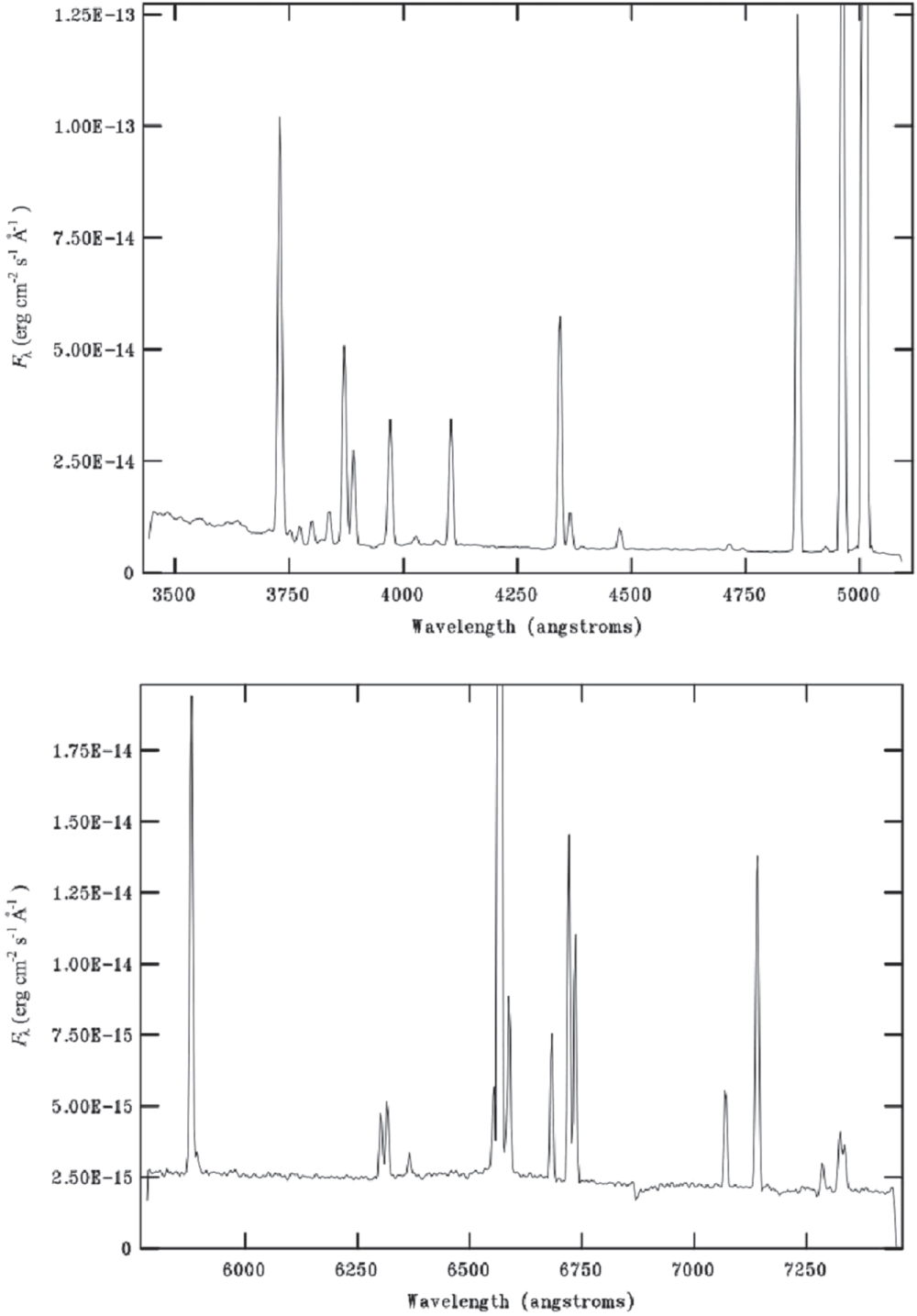
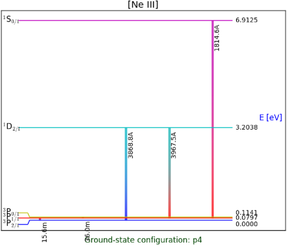
As mentioned in Section 4.2, the electron velocity distributions in H ii regions and PNe are very close to Maxwellian, ruling out the possibility that κ distributions can account for the large ADF values observed (Ferland et al. 2016). Therefore, other causes should be found to explain the t2/ADF problem.
Nevertheless, κ distributions have been used in many papers on gaseous nebulae, both estimating them from observations or computing atomic data for different κ values. The κ distributions can be represented by temperature inhomogeneities; the t2 needed can be obtained by the following expression:

Therefore, values derived from observations or used in atomic physics computations, in the of  range, correspond to the observed values of
  (Peimbert & Peimbert 2013; Ferland et al. 2016).
7.2. Chemical Inhomogeneities
Tsamis et al. (2003), Tsamis & Pequignot (2005), and Stasińska et al. (2007) suggested the presence of metal-rich droplets produced by supernova ejecta as predicted in the scenario of Tenorio-Tagle (1996). These droplets do not get fully mixed with the interstellar medium until they become photoionized in H ii regions and they could be responsible for the ADF problem in H ii regions. Moreover, these droplets, if present, had to be denser and cooler than the surrounding material in H ii regions. Based on high-quality observations of multiplet V1 of O ii of 8 galactic H ii regions and one extragalactic H ii region, Peimbert & Peimbert (2013) find that the signature of oxygen-rich droplets of high density and low temperature is absent, ruling out the possibility of chemical inhomogeneities in these H ii regions.
Similarly, Peimbert et al. (2014), based on high-quality observations of multiplet V1 of O ii in 16 galactic planetary nebulae, find ADF values in the 1.42 to 9.67 range (including NGC 6153 with an ADF of 9.67). They also find that there is no sign of low-temperature, high-density droplets, implying that these objects are chemically homogeneous. For chemically inhomogeneous PNe, the relatively metal-rich regions are expected to be cooler than the relatively metal-poor ones.
Alternatively, Corradi et al. (2015), García-Rojas (2016), García-Rojas et al. (2016a, 2017), Jones et al. (2016), McNabb et al. (2016), and Wesson et al. (2017, and references therein) have found a group of PNe that show ADF values in the 10 to 80 range. This group includes Haro 2–33 (Hen 2–283), Fg 1, NGC 6778, NGC 6337, NGC 6337, Pe 1–9, MPA 1759, M1–42, Hf 2–2, Abell 63, Abell 46, and Abell 30. This group corresponds to binary stars that after a first ejection of gas produce a second one with a very small mass but with a very high overabundance of O/H relative to the first ejecta. The ADF in these objects is strongly centrally peaked. They propose that these large ADF values should be explained in the framework of close binary evolution and discuss the possibility that these systems could have gone through a common envelope phase.
Some giant extragalactic H ii regions include WR stars and SNe remnants that will produce chemical inhomogeneities, like NGC 2363 (González-Delgado et al. 1994).
7.3. Deposition of Mechanical Energy (Shocks and Turbulence)
Peimbert et al. (1991) suggest that the high t2 values observed in PNe and H ii regions might be due to the presence of shock waves.
Peimbert et al. (1995) find that T(C++), the temperature derived from the C iii I(1906 + 1909)/I(4267), ratio is in general considerably smaller than the T(O++) temperature derived from the I(5007)/I(4363) ratio. They also find that the objects with highest  values are those that show large velocities and complex velocity fields, and consequently suggest that the deposition of mechanical energy by the stellar winds of the PNe is the main responsible for the temperature differences.
González-Delgado et al. (1994) propose that stellar winds from WR stars play an important role explaining the high t2 values derived for the giant extragalactic H ii region NGC 2363.
Stasińska & Schaerer (1999) find that photoionization models of I Zw 18 yield too low [O iii] λλ4363/5007 ratio by about 30%, relative to the observed value. This difference might be due to the presence of shock waves and turbulence. Similar results were obtained by González-Delgado et al. (1994) and Luridiana et al. (1999) for NGC 2363, Luridiana & Peimbert (2001) for NGC 5461, and Relaño et al. (2002) for NGC 346.
O'Dell et al. (2015) discuss the presence of stellar outflows in the Orion Nebula. Outflows can produce shocks and turbulence. Arthur et al. (2016) discuss the presence of turbulence in the Orion Nebula. The Orion Nebula is an H ii region ionized mainly by an O7 star, while many of the giant extragalactic H ii regions, for example NGC 5471 (Skillman 1985), I Zw 18 (Skillman & Kennicutt 1993), and NGC 2363 (González-Delgado et al. 1994), present evidence of large velocity winds probably produced by Wolf-Rayet stars and supernovae. These powerful outflows might be partly responsible for the higher t2 values derived for these objects than those observed in the Orion Nebula.
7.4. Time-dependent Ionization Might be Important for PNe, but Not for H ii Regions
When a photoionization front passes through a nebula it heats the gas above the steady-state value, and some time is needed to reach thermal equilibrium. When the stellar ionizing flux decreases, the outer regions of the nebula become isolated from the stellar radiation field and will continue cooling before fully recombining, creating cold partially ionized outer regions (this might be the case in NGC 7009).
7.5. Density Inhomogeneities
Extreme density inhomogeneities are present in most PNe, as can be seen from optical images. Density inhomogeneities produce temperature inhomogeneities, because when the density is high enough, CELs can be de-excited collisionally reducing the cooling efficiency of the forbidden lines.
Viegas & Clegg (1994) have discussed this possibility and find that for typical, chemically homogeneous PNe, this effect is of the order of  or less. For chemically inhomogeneous PNe, the effect of density inhomogeneities is crucial.
For steady-state photoionization models, moderate density inhomogeneities are not very important; however, for time-dependent processes, the regions of higher density will reach equilibrium sooner than those of lower density.
The relevance of the density inhomogeneities can be estimated from the filling factor (see Equation (14)), which is almost always considerably smaller than one (e.g., Mallik & Peimbert 1988).
7.6. Shadowed Regions
Mathis (1976) proposed the ionization by diffuse radiation of shadowed regions, which are those regions ionized by photons not directly coming from the ionizing star. The shadowed regions in PNe are expected to have a lower temperature than that of the directly ionized regions from the central star. For the Helix Nebula, NGC 7293, Cantó et al. (1998) and O'Dell et al. (2005) estimate the temperature of the shadowed regions to be from one-half to two-thirds that of regions ionized directly by the central star. This process is present, but it is not the main one producing temperature inhomogeneities. For NGC 7293, the high-density knots cover only about 0.05 of the total solid angle (covering factor) as seen from the central star; this could contribute to t2 with about 0.005–0.010.
7.7. Cosmic Rays
Based on the very small upper limit that they obtain for the I(4686, He++)/I(Hβ) ratio, Peimbert & Goldsmith (1972) conclude that cosmic rays are not important in the heating rate of the Orion nebula; they also suggest that the observed I(4686)/I(Hβ) ratio in some extragalactic H ii regions might be due to cosmic ray ionization. Giammanco & Beckman (2005) propose the ionization by cosmic rays as a key mechanism acting in giant H ii regions.
7.8. Spatially Distributed Ionization Sources Inside H ii Regions
Ercolano et al. (2007) study the effects of spatially distributed ionization sources on the temperature structure of H ii regions. They find that metallicity indicators calibrated by grids of spherically symmetric photoionization models may suffer a systematic bias due to their dependence on the ionization parameter of the system. The O/H values derived by not considering this effect produce underestimates in the 0.1 to 0.3 dex range. These errors are likely to represent the worst case scenario, nevertheless their magnitude and systematic nature do not allow them to be ignored.
7.9. Overestimation of the Intensity of Weak Emission Lines
Rola & Pelat (1994) have shown that the intensity of a weak line with a S/N smaller than 5 is overestimated. This effect might be present in the observations of oxygen and carbon RLs that in a given object are typically three orders of magnitude fainter than the brighter RLs of H. This intensity overestimation could also be present in the [O iii] 4363 line that is typically two or three orders of magnitude fainter than the [O iii] 5007 line. The overestimation of the oxygen RLs produce higher O/H abundances than the real ones, while the overestimation of [O iii] 4363 produces higher  and lower O/H abundances than the real ones. These two results increase spuriously the ADF values. To avoid this possibility, it is important to measure line intensities with a higher than 5 S/N.
7.10. Magnetic Reconnection
García-Segura et al. (2001) propose that the multiple, regularly spaced concentric shells around some PNe could be due to the effects of a solar-like magnetic, cycle with a periodic polarity inversion in the slow wind of an asymptotic giant branch (AGB) star. Presumably these shells of alternating polarity could give rise to magnetic reconnection processes once that they are compressed in the formed PN (i.e., in the swept-up shell). Magnetic fields have been measured in the torus surrounding K3–35 (Miranda et al. 2001); also, the presence of a magnetic field has been inferred in the PN OH0.9 + 1.3 (Zijlstra et al. 1989) and in the pre-planetary nebula IRAS 17150–3224 (Hu et al. 1993).
7.11. Summary on t2
From the previous discussion, we consider that the best abundance determinations are those derived from the oxygen and hydrogen RLs and that the t2 values derived from observations should be used to estimate the abundances derived from forbidden lines of the other elements.
H ii regions have t2 values in the 0.02 to 0.12 range, with a typical value of 0.045, and ADF values in the 1.5 to 3 range with a typical value of 2. We conclude that probably in H ii regions, the main source of temperature inhomogeneities is due to the deposition of mechanical energy by shocks and turbulence produced by stellar winds, including those winds due to SNe and WR stars in giant extragalactic H ii regions.
We divide PNe in two groups: (a) classical PNe with homogeneous chemical composition and (b) PNe with inhomogeneous chemical composition.
Classical PNe have the following properties: (a) they do not have gaseous inclusions of high density and low temperature; (b) they have t2 values in the 0.024 to 0.128 range with a typical t2 value of 0.065; (c) they have ADF values in te 1.4 to 10.0 range with a typical value of 2.3; and (d) they have typical ionized masses in the 0.05 to 0.40 M⊙ range (e.g., Mallik & Peimbert 1988).
PNe with inhomogeneous chemical composition have the following properties: (a) they do have inclusions of high density and low temperature in the gaseous envelope, possibly the result of close binary evolution; (b) their O/H values decrease from the central star outward; (c) they present large temperature inhomogeneities that cannot be analyzed with the t2 formalism in a one-phase model; (d) their ADF values are in the 10 to 100 range; and (e) they have typical ionized masses of about 0.01 M⊙.
For chemically homogeneous PNe, the best abundance determinations are those derived from oxygen and hydrogen RLs. We also conclude that probably the main source of temperature inhomogeneities in PNe is due to the deposition of mechanical energy from strong stellar winds.
For chemical inhomogeneous PNe, the best approach to determine the chemical abundances is to construct two-phase models, but still a particular kind of t2 should be considered when fitting such models. By their very essence, such models will not have a homogeneous temperature; moreover, with inhomogeneous chemistry, the t2 value can be very different for each chemical element and for each ion. Most of this will be directly considered when studying the two phases of the model; however, the hot phase alone is expected to behave similarly to a chemically homogeneous PN, and as such it is expected to have its own particular t2 (and ADFs). Because most of the CEL intensities are expected to come from this phase, the t2 corresponding to the hot phase alone is necessary and should be sufficient to reproduce the behavior of all the optical CELs observed in these objects.
8. Final Remarks
The determination of accurate chemical abundances of PNe and H ii regions is a fundamental problem in astrophysics. The chemical abundances of PNe provide us with constrains for stellar models in the 0.8 M⊙ to 8 M⊙ range. H ii regions permit us to determine the initial abundances with which stars are formed. Both sets of data are fundamental for the study of stellar and galactic chemical evolution.
Also, accurate abundances of H ii regions and PNe are needed to estimate the fraction of the elements embedded in dust grains. These fractions are needed to study the processes of formation and destruction of dust in gaseous nebulae.
Further efforts are needed to obtain data for H ii regions and PNe in galaxies of different types. In spiral galaxies, observations of H ii regions at different galactocentric distances to study which has been the evolution of the ISM as a function of time for these galaxies. The study of very metal-poor extragalactic H ii regions will permit to increase the accuracy of the primordial helium determination; this value is important for cosmology and particle physics.
The ADF problem should be studied further to obtain a consensus on its origin and scope. The same can be said for the high t2 values derived from observations of H ii regions and PNe.
We thank the referee for many excellent suggestions. We are grateful to all those who have worked and are working in this field; they have inspired us over the years. M.P., A.P., and G.D-I. received partial support from CONACyT grant 241732. M.P. and A.P. acknowledge support from PAPIIT (DGAPA-UNAM) grant no. IN-109716. G.D-I. acknowledges support from PAPIIT (DGAPA-UNAM) grant No. IA-101517.
Footnotes
- 1
- 2
- 3
- 4
- 5
- 6
- 7