

Abstract
This work approaches the Michaelis-Menten model for enzymatic reactions at a nanoscale, where we focus on the quasi-stationary state of the process. The entropy and the kinetics of the stochastic fluctuations are studied to obtain new understanding about the catalytic reaction. The treatment of this problem begins with a state space describing an initial amount of substrate and enzyme-substrate complex molecules. Using the van Kampen expansion, this state space is split into a deterministic one for the mean concentrations involved, and a stochastic one for the fluctuations of these concentrations. The probability density in the fluctuation space displays a behavior that can be described as a rotation, which can be better understood using the formalism of stochastic velocities. The key idea is to consider an ensemble of physical systems that can be handled as if they were a purely conceptual gas in the fluctuation space. The entropy of the system increases when the reaction starts and slightly diminishes once it is over, suggesting: 1. The existence of a rearrangement process during the reaction. 2. According to the second law of thermodynamics, the presence of an external energy source that causes the vibrations of the structure of the enzyme to vibrate, helping the catalytic process. For the sake of completeness and for a uniform notation throughout this work and the ones referenced, the initial sections are dedicated to a short examination of the master equation and the van Kampen method for the separation of the problem into a deterministic and stochastic parts. A Fokker-Planck equation (FPE) is obtained in the latter part, which is then used as grounds to discuss the formalism of stochastic velocities and the entropy of the system. The results are discussed based on the references cited in this work.
Export citation and abstract BibTeX RIS
Introduction
The Michaelis-Menten catalysis model is routinely used in biochemistry, as it describes the reaction velocity,  defined as the time derivative of the product. The equation for
  was obtained by Leonor Michaelis and Maud Menten in 1913 [1] and is preceded by Victor Henri [2], who published in 1903 an article proposing that the basis for explaining the phenomenon of catalysis could be a reversible reaction between an enzyme (
 ) and a substrate (
 ), to produce an enzyme-substrate complex (
 ), from which an irreversible reaction could yield a product (
 ) and a free enzyme.
The conditions of the validity of the algebraic equation resulting from this model has been widely studied [3, 4], and a variety of methods have been used to study the dynamics of the reaction [5–7]. From the point of view of stochastic processes, it is worth to mention A. F. Bartholomay [8], who formulated the problem of chemical reactions as a probability density that was a function of time and of the concentrations of substrate and enzyme-substrate complex. He obtained the corresponding master equation and demonstrated that the time evolution of the means of the concentrations match with the non-linear differential equations known in the textbooks of chemical kinetics. Sandra Hasstedt [9] studied the same problem with bivalued variables {0, 1}, to indicate the presence or absence of a single enzyme molecule. Arányi and Thöt [10] developed a similar approach for states with zero or one enzyme molecule but an unlimited amount of substrate molecules. After 1990, the advancements in technology and measurement techniques using Raman spectroscopy and methods of photo-physics and photochemistry [11–13], have made the study of random fluctuations a necessity. In the XXI century the study of stochastic systems has proliferated [14–16] brought to attention to the fact that, in the smaller dimensions inside of the cell, enzymes are subject to random fluctuations due to the Brownian motion, causing random displacements of these, therefore changing the reaction rates. After noting that the number of proteins is also very small, they questioned the description of reactions based in the continuous flow of matter and proposed a formulation in terms of discrete stochastic equations. Puchaka and Kierzek [17] suggested a method named 'maximal time step method' aimed at stochastic simulation of systems composed of metabolic reactions and regulatory processes involving small quantities of molecules. Turner et al [18] reviewed the efforts intended to include the effects of fluctuations in the structural organization of the cytoplasm and the limited diffusion of molecules due to molecular aggregation, and discussed the advantages of these for the modelling of intracellular reactions. In 2008 Valdus Saks et al [19] showed that cells have a highly compartmentalized inner structure, thus they are not to be considered as simple bags of protein where enzymes diffuse as a gas. Also, this type of works has inspired specialists to design drugs, who have initiated studies about the required sizes for better substrate processing. Among these, one analyzed pairs of compartments in cyanobacterias, which contain two compartments named α-carboxysome and β-carboxysome, with dimensions of the order of nanometers [20]. These elements lead us to maintain our position that the analysis of random fluctuations of substance concentrations are relevant in biochemical systems.
While there are many enzyme reactions that can be described by the Michaelis-Menten model, it is better suited for cases that follow two conditions:
- 1.The number of substrate species that can bind to an enzyme is one.
- 2.The system does not exhibit cooperativity, therefore the curve of the reaction velocity, as a function of substrate concentration, has a hyperbolic shape.
It is to be expected that random phenomena take greater importance when experiments are carried out at a nanoscale, therefore, it is convenient to thoroughly understand the role of random behavior in cases where the number of reactants is of the order of a few thousands or hundreds. When the van Kampen method is applicable, the system under study can be split in two spaces: one for the deterministic solutions of the means of physical variables, and another for the random fluctuations that occur around these mean values. Amid the results found until now, there is the fact that the probability density of the random fluctuations can be described adequately with a gaussian distribution. In summary, each physical system has a state space associated to it, such that a point in a state space corresponds to a specific set of values for all the system variables.
The objective of this work is to calculate the entropy of fluctuations and present kinematics that describe the behavior of these fluctuations from the point of view of their state space, given the name of fluctuation space. We introduce various stochastic velocities and take advantage of two of these to describe the regions of higher and lower probability. It will be shown that, during the course of the chemical reaction, an entropy of fluctuation arises that presents two characteristics:
- 1.The initial increment is positive, which guarantees the spontaneity nature of the reaction.
- 2.There is a subsequent decrease in entropy, which in turn reveals two aspects:
- a.There exists a source of energy in the process.
- b.This decrease in the change of entropy translates into the heat capacity at constant pressure,Cp , is negative in the catalysis. This is a result that has been confirmed in previous literature.
The stochastic velocities surged as part of the efforts to understand quantum phenomena as a probabilistic problem [21–24]. However, the mathematical expansion is valid for any stochastic phenomenon that can be described by diffusion equations. These velocities have been useful to study the active Brownian motion by one of the authors of this work [25] and now this is applied to the field mentioned in this section.
This article is organized as follows:
We begin by defining the physical system and present the results of a simulated reaction using the Gillespie algorithm. In the following section, based on the graphs obtained from it, we review the theory developed by Bartholomay, which is used to split the state space in two: one for the average concentrations and another for their fluctuations (the latter one receiving the name of fluctuation space). In this same section we clarify what is understood by a state of equilibrium in this work, and its difference with the stationary state under study.
In the next section we analyze the behavior of the state points in the fluctuation space obtained previously and do a short review of the stochastic velocities formalism, as well as obtain the expression for the entropy in this system. We pay special attention to the form of these velocities in time dependent Ornstein-Uhlenbeck processes. We examine what it means to reach a state of equilibrium in the simulated reaction, and the conduct of the probability density of the state points in the fluctuation space during the quasi-stationary state.
We then retake the discussion of the entropy, performing an estimation of its value at different points in time of the reaction. We find that, during the evolution of the reaction, the Michaelis-Menten model is capable of describing an expected decrease of the entropy of the system.
We close this article by discussing the results obtained and our conclusions.
Physical system
The physical system under consideration is the chemical reaction posed in the introduction section. During the time interval  enzyme and substrate molecules exist without interaction within a fluid that serves as a medium that is in thermodynamic equilibrium. At time
  the system suffers a change that gives way to the start of the reaction, an event that could be, for example, the stirring of the fluid with the enzymes and substrate molecules. During the interval
  the system undergoes the process of a catalytic reaction until all substrate molecules have been depleted.
We started by simulating a reaction using the Gillespie algorithm [26]. The number of enzymes ( ), substrate (
 ), enzyme-substrate complex (
 ) and product (
 ) are under observation. One hundred realizations are carried out with the following initial conditions:
  The reaction rates were taken from the work by Weilandt et al [27] and selecting the special case where the reaction is irreversible, thus
  In this work the notation used for the reaction rates are presented in table 1.
Table 1. Reaction rate used in the simulation.

| 1.52 × 10⁵ |

|
| k2 | 10 |

|
| k3 | 22 |

|
| r | 6.5579 × 10⁻⁵ |

|
| kM | 2.105 × 10⁻⁴ | (M) |
The simulation results were data structures for ( ), where
  is the time between reactions. An example of a time evolution of
  and
and  as it progresses towards a stationary state is given in figure 1.
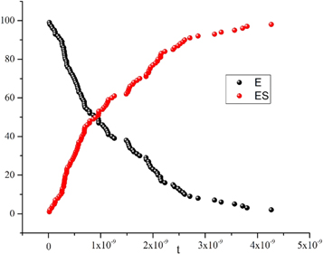
Figure 1. Time evolution of the number of enzyme molecules (black) and ES complex (red) reaching stationary states. One realization with the Gillespie algorithm. Initial conditions: E = 100, S = 4900, ES = 0, P = 0.
Download figure:
Standard image High-resolution imageWe found that as the reaction progresses, the number of enzymes decreases to almost zero due to them having transitioned to the enzyme-substrate complex state. Once in this state, the quantity of  s kept almost constant in time. The amount of
  decreases as it is consumed to form
  and when the process is nearing depletion of
  the same occurs to
  returning the amount of free enzyme
  to its initial value. The evolution of
  and
and  is shown in figure 2.

Figure 2. Time evolution the number of enzyme molecules (black) and ES complexes (red). The number of ES go to zero. One realization with the Gillespie algorithm. Initial conditions: E = 100, S = 4900, ES = 0, P = 0.
Download figure:
Standard image High-resolution imageBetween the initial and final stages exists a stage that called the quasi-stationary state of the chemical reaction. This is presented in figure 3 and is the regime that will be addressed in greater detail in this work.

Figure 3. The number of ES complexes is almost constant. This is the state considered as stationary in this work. Average over 100 realizations with the Gillespie algorithm. Initial conditions: E = 100, S = 4900, ES = 0, P = 0.
Download figure:
Standard image High-resolution imageFigures 1 and 2 show the stochastic nature of this process, and these random fluctuations are the focal point of our work. An adequate treatment for this kind of problems was developed in the past; this is presented in the section below.
One of the results obtained predicts that the profile of the mean of the ES complex is a decreasing curve. This occurs when the product is reaching its constant value and the amount of substrate is nearly depleted. We will also demonstrate that this is what is called the state of equilibrium.
Master equation and the Van Kampen omega expansion
The usual mathematical treatment sets off from the consideration of a process where a number of  enzyme molecules and
  substrate molecules react, first to form an enzyme-substrate complex in a reversible reaction, followed by an irreversible reaction that can form a product plus a free enzyme. We model this system through 4 amounts that at a given time
  have:
have:  enzyme particles,
  substrate particles,
  enzyme-substrate complexes, and
  product particles.
Two laws of conservation are followed:
- 1.The number of enzyme molecules at any given time are conserved and can be described by:

- 2.The number of substrate molecules at any given time are conserved and can be described by:


From above follows that there are only two independent variables, therefore  are taken as the state variables that evolve with time, and to introduce
  as the probability that there are
  substrate particles and
  enzyme-substrate complexes at time
  From now on these will be called
  to ease reading and to connect with the notation used in [28]. The time evolution equation of
  is obtained on the basis of three transitions that can occur in the state space representable in a two-dimensional plane, as shown in figure 4.
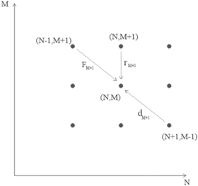
Figure 4. State space. The number of complexes M versus the number of substrates N. The arrows show the transitions needed to build the master equation.
Download figure:
Standard image High-resolution imageThe probability  can be calculated considering the conservation of probability. Each term consists of two factors, such that each factor is the probability of an independent event. For instance, in the event where the state transitions from
  to
to  in the interval
  considers the product of the probability of the state to be at
  at time
  and the probability of the transition to be towards
  A similar argument is applicable for each of the three transitions drawn in figure 4. There also exist the passive transition, that consists of the system already being at state
  at time
  and stays in that state during the time interval
  The general formulation of this can be consulted in [28]. The resulting master equation is

where

with step operators


The van Kampen omega expansion allows one to separate the state space represented in figure 4 in two distinct spaces, one for the deterministic side of the problem, and another for the random fluctuations. For this purpose, the next intensive variables are defined:

with  It is important to note that, while it is common practice to define concentration as the quotient between the number of molecules within a volume, in this work it is defined in respect to the total number of reactants in the system. The relation between both ratios is a constant.
The pair  represent the deterministic conduct (also called the macroscopic description) of the particle densities (concentrations), and the pair
  are their respective random fluctuations.
The step operator acts as shown in equation (6) below:

Such that the action of this step operator causes the change  There is an analogous expression for
  Working with an arbitrary function, of which the second derivatives exists, from their Taylor expansion follows that an approximation for the operators can be expressed as:

These will be used in expression (4), along with transition rates 
If one is looking for a probabilistic treatment where a well-defined probability density is obtained, in the sense that it is non-negative for every value of time  in all the fluctuation space
  the only option is to cut (7) at its second order. Higher order expansions allow working with statistical moments or cumulants, but the pseudoprobability being used is not well defined; non-negativity is only recovered if all the terms in the series are used, in other words, if
  is of the form shown in the expression below:
The other three operators involved would also have to have analogous expressions. In other words, according to the Pawula theorem, the expansion should stop after the first term or after the second term. On the contrary, it must contain an infinite number of terms, for the solution to the equation to be interpretable as a probability density function [29].
The transition rates are usually introduced by means of the law of mass action, resulting in

with  as the reaction rates given by the Arrhenius law. The description in the state space
  is recovered by considering
  in
in 
Substituting (5) in (8) and rescaling  results in


Also, now the probability  has the following functional dependence for every pair of

Substituting (7) and (9) to (11) in (4), the right-hand side of the master equation (3) takes the following form:

The left-hand side is also rewritten as:

Substituting (13) and (14) in the master equation, and comparing terms with like coefficients it is possible to obtain:
For 

For 

The equations for the deterministic part of the problem, also called the macroscopic part, can be obtained through  and the partial differential equation that allows the study of the random fluctuations can be obtained through
  The procedures for these are widely covered in the literature [24]. From here onwards we will be using them in the context of the notation initially proposed in this work as was done in [28].
Deterministic equations
The equations for the mean substrate concentration,  and the mean concentration of enzyme-substrate complex,
  that describe the macroscopic part are:

This approach is versatile enough to be of use at any enzyme-substrate ratio, since these differential equations can be solved numerically for different initial conditions; but it will be used with the usual proportions of reactants found in in-vitro experiments, where the initial substrate concentration is much greater than the initial enzyme concentration. The logic behind this is that smaller quantities of enzyme can catalyze much larger quantities of substrate, thus it is a topic of efficiency; however, this is not the only situation that can be studied in the laboratories. Albe et al [30] report the progress of a chemical reaction with different enzyme-substrate ratios, including cases where these ratios are inverted, so that the amount of enzyme exceeds that of the substrate.
Equations (17) can take a very practical form when multiplied by  and one can define the evolution parameter
  with units of
  The resulting expressions are:

Where  is an efficiency parameter that measures the rate of dissociation of the
  complex that is not transformed into product.
Quasi-stationary state
The quasi-stationary state that is of interest in the in-vitro experiments is obtained through the condition that the density of enzyme-substrate complex changes very little across time, which is mathematically expressed as  This is the topic of discussion in this subsection.
In terms of the densities, the conservation laws take the form of

Where  and
and  are the densities of the enzyme and the product, respectively. It is possible to demonstrate that the time evolution equations can be obtained through the following expressions:

Introducing the quasi-stationary condition in the time evolution equation of  in (17) results in

The conservation laws yield the relation  such that

where  and receives the well-known name of the Michaelis-Menten constant.
Denoting as  the rate of growth of the product density
  one obtains

The in-vitro experiments are performed with amounts on the order micromoles. In such cases the behavior observed is of a slow decrease of the functions  and
and  It is then where the condition of
  is applicable.
From the deterministic equation for  in (18) results

One can obtain the following expression for the mean concentration of enzyme-substrate complex:

Using de definition  and the time evolution of
  in (20), the demonstration of the following expression is straightforward.

Where  The usual notation is recovered by simply rewriting
  as
as ![$\left[S\right].$](https://content.cld.iop.org/journals/1402-4896/96/8/085006/revision3/psabfd65ieqn100.gif)
Equilibrium state
It is common practice to indistinctively use the terms 'stationary' and 'equilibrium' as synonyms, but it is imperative to establish a clear distinction between them. This section is dedicated to this purpose, showing the difference between a stationary state achieved in in-vitro experiments and the equilibrium state. This latter one corresponds to the mathematical condition:

such that the following equations are followed:

The algebraic solution is  it corresponds to the complete consumption of the substrate and enzyme-substrate complex. It is for this reason that the state of equilibrium is only attainable when all the substrate has been consumed, such that only the initial amounts of free enzymes and the product remain in the system.
It is possible to study the stability of the equilibrium state. Linearizing the differential equations around  results in:
To ease reading, we introduce a shorter notation:

Thus, the eigenvalues of the matrix above are given as:
The transition rates and initial conditions are defined positive, this results in the eigenvalues satisfying the inequality:  The fundamental solutions
  generate the most general solution:
Which will always converge towards the equilibrium state. This mathematic expression explains the profile of the curve for the  complex seen in figure 1 and the decreasing stage shown in figure 14.
Analysis of the random fluctuations
General solution
The following equation is called the Fokker-Planck equation (FPE):

The expression above describes the probability that the fluctuation of substrate concentration takes the value  and the fluctuation of enzyme-substrate complex concentration takes the value
  at time
  The systematic term can be written as

Where  is the flux of random concentration fluctuations of
  and
and 
And its general solution [31] is a gaussian function of the form:

with  as the self-correlation matrix, and
  as its inverse. This is the matrix that contains the variance of the random concentration fluctuations of
  and
and  as well as their correlations.
In the case under study, the elements of  and
and  are given by:


Given a physical magnitude  that is relevant to the system, its mean can be calculated by:

The time evolution equations of the mean of the fluctuations of the concentrations of  and
and  take the form of:

and the time evolution equations for the self-correlation functions are:

Defining ![$\vec{{\rm{\Xi }}}\left(t\right)=\left[{{\rm{\Xi }}}_{11}\left(t\right),{{\rm{\Xi }}}_{12}\left(t\right),{{\rm{\Xi }}}_{22}\left(t\right)\right]$](https://content.cld.iop.org/journals/1402-4896/96/8/085006/revision3/psabfd65ieqn121.gif) and
and ![$\vec{D}\left(t\right)=\left[{D}_{11}\left(t\right),{D}_{12}\left(t\right),{D}_{22}\left(t\right)\right],$](https://content.cld.iop.org/journals/1402-4896/96/8/085006/revision3/psabfd65ieqn122.gif) the equation above can be rewritten as follows:
the equation above can be rewritten as follows:

where

Defining the entropy of fluctuation of the concentrations of  and
and  as
as

Substituting the general solution in the expression for the entropy (35), results in expression (36) seen below:

Given two temporal points such that  the change in entropy is

so, the condition of  translates into the following condition:

Expression (38) will later be utilized to confirm that the entropy of fluctuation decreases when the reaction is taking place. Expression (27) provides the mathematical form of the time dependent probability density for the fluctuation variables which, as will be shown in the numerical example in a later section, performs a clockwise turning motion as the reaction progresses. This result showcases the importance of fluctuations in the dynamics of catalysis; therefore, in-depth study of this topic is relevant.
If the phenomenon is analyzed using the dynamics of stochastic velocities, the behavior observed can be better understood. Thus, the section below is dedicated to the introduction of this formalism that may prove useful to the uninitiated reader.
Stochastic velocities
The time evolution of the fluctuations can be described by the motion of a state point  It is common to assume that its study is completed once its behavior has been formulated, as we did in the previous section. We will see that it is possible to add new knowledge to better understand the behavior of the state point
In this section we present an intuitive approach to stochastic velocities. We begin with an analysis of the difficulty found when attempting to define velocities in stochastic processes. The typical example given of a stochastic process is the Brownian motion; this describes the conduct of a micrometric mass floating inside a liquid at temperature  Seen through a modern video camera, its movement takes place in two dimensions, but for ease of writing mathematical expressions, we consider only one dimension. The model treats the Brownian particle as if it is a point mass, and due to the movement possessing random behavior, each point
  has a time dependent probability associated to it. This probability is a probability density function, denoted as
  such that a given interval,
  on the line of accessible positions, the expression
  yields the probability of the particle being found within that interval at time
It can be demonstrated that  follows an equation of the form shown below:

where  is named the diffusion coefficient. With the initial condition
  the solution obtained for (39) is

In this case, the probability densities evolve with time. From (40), the statistical properties  and
and  can be demonstrated. It is important to note that the mean movement is zero and that the standard deviation changes with time as
  In the approach presented by Paul Langevin in 1908, the Second Law of Newton is applied to a Brownian particle of mass
  with a force
  acting upon it; plus a friction force proportional to the velocity,
  plus a stochastic force,
  with the following properties:

where  is a constant. There are technical reasons for calling white noise a random magnitude that displays these properties. The fundamental dynamic law resulting from this is called the Langevin equation, and is written as shown below:

Using the method of moments, one obtains similar results for the Brownian motion. If the trajectories as functions of time  are to be plotted, the resulting graphs would present functions with very sharp peaks and valleys, therefore one can perceive intuitively that there would be problems when attempting to define the displacement velocity as
  Next, we will focus on this dilemma with close attention.
In mathematical terms, the Weiner process has been defined to formalize the events that follow the Brownian motion. Taking as a starting point the case where  and denoting the process as
  the postulated properties are:
- 1.
- 2. is continuous.
- 3. has independent increments, that is to say, if it follows that then the differences and are independent random variables.
- 4. is a random variable with normal distribution of mean and variance


In rigorous terms, equation (42) presents a difficulty that is analyzed next. Using the traditional concepts of defining the rate of change in a trajectory  we take the quotient of finite increments:

but from the fourth postulate one must have  where it follows that
  Therefore, the quotient diverges in the limit
  consequently, it is impossible to define the rate of change through traditional methods.
For the issue encountered above, instead of using the Langevin equation, as it was originally formulated, it is better to consider an approach using finite differences to suggest an equation that avoids the use of derivatives and translates all calculations to integrals, giving place to two types of integral calculus: that of Kiyoshi Ito and of Ruslan Stratonovich [32]. A less known option is the one developed by Edward Nelson, based in a system of averages over the realizations of the stochastic processes, and gives place to the concept of stochastic velocities [22, 33]. These have been used to describe quantum phenomena from a stochastic perspective, giving rise to a line of work called stochastic mechanics. In this work we take advantage of the mathematical tools developed and use them in our topic of interest. The condition is that the stochastic process must be describable by means of Fokker-Planck equations (FPE) [25].
When an ensemble is associated to a stochastic process  a state space of dimension
  is available in which a point at a time
  corresponds to each member of the ensemble. A large number of members of the ensemble produce a cloud of points that move at random as time progresses; this idea allows the introduction of an analogy with a gas, such that it is possible to include in the description some properties typical of fluids. One of these is that of vorticity, which lets us know if the cloud of state points tends to rotate, or if it behaves like a fluid whose velocity is irrotational. This gives us the opportunity of using this concept to analyze the manner with which the agitation of this cloud of state points occurs, and with it establish a difference between a stationary process and that of a process at equilibrium. The former abides to the condition that the statistical moment of order
  must be time invariant:

while the latter also follows the condition that each of the possible transitions must be balanced out by a transition that occurs on the opposite side. This condition is given the name of detailed balance. If the detailed balance is not present, then the cloud of state points tends to rotate, therefore, the use of the concept of vorticity contributes to the understanding of the dynamics of the gas cloud. Vorticity is defined as the curl of the velocity thus it is necessary to revise this point.
Smoothening the trajectory using a moving average
The mean over the realizations, as originally developed by Nelson, can be understood with the concept of moving averages used in the study of time series. In this section we introduce these concepts.
Let  be a stochastic process that occurs inside a state space
  and let the points
  such that they are reached by some realizations of the stochastic process
  at times
  respectively, where
  Let the increments be
  see figure 5.

Figure 5. The state space  The neighborhood of the point
 is the region of interest where we determine the state points going inside or outside. One can arrive to the definition of the access and exit velocities if the times are considered. The stochastic process
  can jump to points:
  The velocities are defined depending on the jump. Each point is reached at times
  The increments considered in the definitions are:
Download figure:
Standard image High-resolution imageNext, we will explain the relations that must be followed between the time intervals involved in the description; for that purpose, we continue using the Brownian movement as a case study. Suppose a camera capable of registering the random movements of a state point; due to the difference in mass, the collision of a single molecule against the Brownian particle does not produce an effect that is registerable by the lab instrument. What moves the Brownian particle is the difference in the number of collisions that it receives because of the random fluctuations of the density of particles comprising the surrounding medium. By this manner, the path traced by the Brownian particle, as observed by a camera recording through an optical microscope, are polygonal shaped. However, because of the easiness in the mathematical language, we say that a collision occurs each time there is a change in the path taken by the particle of interest.
There are three instants of time that are relevant in this approach:
- 1. the time required to accumulate enough collisions capable of causing a registerable random change in the path of the particle.
- 2. the time that passes between two successive frames captured by the camera. If is too short, the displacements registered may follow the relation as is the case in classical mechanics; but it is more common to find in the Brownian case. For the latter conduct it is necessary that
- 3.t, the time necessary to smoothen trajectories by the moving averages method. To study the movement of the state points, the stochastic trajectories are smoothed by introducing moving averages; these are calculated in time intervals that must be long enough to include various spikes of the trajectory, as can be seen in figure 7, but also short enough that the camera registering the data cannot tell that the trajectory has been smoothed.


Therefore,  must be followed. This regime is called the coarse grain time scale, as shown in figure 6 below.

Figure 6.
 is the time required to accumulate enough collisions to achieve a random motion.
  is the time between two successive images, or measurements, taken by a camera, or measuring device.
  is the time required to calculate a moving average.
Download figure:
Standard image High-resolution imageThe moving average of  points is defined as
  where
where  takes values such that the sum is not out of the bounds of the interval. For continuous signals, the moving average is defined as:
  We now set out to study the derivative of a function
  For this purpose, we establish a set of times expressed in (45) below:

and considering finite increments of the function 
 with
with  one can write:

Rearranging and multiplying by  gives
gives

This expression receives the name of coarse grain time derivative. Notice the incorporation of the sum of finite differences inside a moving average within an interval of width  Once the smoothening process has been applied, the resulting trajectories can be studied using the usual tools of calculus. An illustrative example is given in figure 7.

Figure 7. The result of the smoothening process is a curve without the spikes that are characteristic of the Brownian motion.
Download figure:
Standard image High-resolution imageThe study of smoothened stochastic functions
Points in the state space and a statistical description of their movement
Suppose a statistical ensemble of equally prepared experiments at a macro scale. Each of these carry out a realization of the stochastic process  At a given point in time, we have a cloud of points whose number is theoretically infinite. If one is to let the clock run out, a static image (like that of a photograph) would be substituted for a series of images of points moving at random, similar to a swarm of mosquitos swirling in summer. These will enter and exit of the previously marked region
  as seen in figure 5. The question that follows is: How many points enter or exit
  in a second? This problem is similar as counting the number of smoke particles in a given region of space.
The concept of systematic velocity, which has already been presented, measure the net number of state points that cross  per second.
Systematic derivative and systematic velocity
We define the systematic derivative as the mean over the ensemble of all the realizations

To have an analytical representation of the previous definition, we introduce various hypotheses that lead to the Taylor series expansion. The hypotheses are:
- The stochasticity of the physical phenomenon is introduced by a source that is: stationary, isotropic and homogenous.
- The second statistical moments of the increments and are such that they follow:


The diffusion matrix can be defined as

or also as

Notice that the increments grow as  so that the average that appears in the definition above grows as
  It also must be noted that the products of increments appear as coefficients in the second order derivatives of any function
  expanded using Taylor series.
To work at higher orders of ( ) would involve considering Taylor expansions with derivatives of orders of
  although it is mathematically possible, there exist a restriction when the problem is translated to determining the probability
  by means of a partial differential equation. The function
  that satisfies an equation of order higher than 2 ceases to be defined as nonnegative for all
  and
and  therefore it cannot be interpreted as a probability density function.
In vector calculus, a function  has a total time derivative that is of the form:

where  is the velocity. The expression above is called the convective derivative.
This concept can be adapted to the case where the function  depends on a stochastic process
  This is the systematic derivative:

such that

Access velocities, of exit and of diffusion
In fluid dynamics appears the phenomenon of swirls, or eddies, that cannot be understood with the systematic velocity alone; an illustrative example would be the that of cigar smoke traveling upwards through the air. To approach this topic let us consider a point  in the state space and both displacements,
  and
and  as shown in figure 5. We have the next relations:

If  is a state point contained in vicinity
  it is understood that the displacement towards
  in a time interval
  is related to the exit of state points. Likewise, the displacement from
  towards
  also in a time interval
  is related with the entry of state points into vicinity
Let us suppose we track a state point whose route is as follows:
- At instant the state point is located at
- At instant the state point is located at


Separating by components and working them individually, one can obtain

We now consider the physical magnitude of the system denoted as  To treat the displacement from
  to
to  the function is expanded in Taylor series as shown below:

such that repeated indexes indicate a sum.
In the same fashion, one can study the displacement from  to
to  resulting in:

The difference between  and
and  is:
is:

It is possible to find that the next relations are followed:

Such that (59) can be written as:

Multiplying by  and calculating the mean results in

From (64) we have that the coefficient of the first derivative with respect to the position, is the ith component of the systematic velocity,  which has been previously found. We also find the following:

Also, the expression  is the systematic derivative of
  thus, we have:

From (64) is easy to identify the systematic derivative operator as:

If one takes as a special case the identity function:  the expression is reduced to the systematic velocity in vicinity
Adding (57) and (58), it results:
Rearranging, multiplying by  and averaging, one obtains:

The term that accompanies the first derivative with respect to the positions is used to define the diffusion velocity in vicinity 

Which is useful to measure the stirring that the state point undergoes in each subset  in the fluctuations space. We can back up this definition if we add the systematic velocity and the diffusion presented above, resulting in:

Which can be interpreted as a total velocity measuring the mean path of state points from  to
to  in the time interval
  In that case

such that the cigarette smoke phenomenon can be described in terms of two velocities, one of translation and other of swirling for each of the  vicinities in the fluctuation space.
With these conceptual tools, one can identify the operators that allow the calculation of the velocities mentioned in this work. Combining results, we find the next expression:

where

With the elements considered up until now, we identify the left-hand side as the stochastic derivative, or of diffusion, of the function  and identify the operator of the stochastic derivative as

such that

To study the exit velocity,  we study the displacement from
  to
to  in a
in a  time interval. For this purpose, we reuse the Taylor expansion given in (57) and rearrange it as:
Multiplying by  and calculating the mean

Defining the  -th component of the exit velocity as follows

and identifying that

thus, we have

Defining the left-hand side as a forward derivative of function  and introduce the forward operator as:

Such that we represent the forward derivative as  In the case when
  one obtains the
  -th component of the exit velocity in vicinity

Finally, one can relate the entry velocity with the translation of the state point from  to
to  in time interval
  (see figure 5). Now consider the Taylor series expansion:

Rearranging, multiplying by  and calculating the mean:

Defining the ith component of the entry velocity in vicinity  as:
as:

and identifying

It is possible to rewrite (81) as:

Defining the backwards derivative operator as

And rewriting (84) as

Once again, if  one can obtain

which is the ith component of the entry velocity in vicinity 
Combining operators
Passing the operators through an algebraic process, one can obtain the following expressions:


If we were to add (88) and (89), then multiply by 

Defining

we have

Now, calculating the difference between (88) and (89) and multiplying by 

such that it is convenient to define:

So (93) can be rewritten as:

The stochastic velocities provide a description at the level of vicinities such that it is possible to calculate a variety of means previously mentioned. Table 2 summarizes the previous results:
Table 2. Stochastic velocities. Notation and associated operator.
| Velocity | Notation | Operator |
|---|---|---|
| Access entry |

|
|
| Exit |

|
|
| Systematic |

|
|
| Diffusion |

|

|
In their current form, their usefulness is not very clear. In the following section we will see a version of these that allows us to study the quasi-local conduct of the state points in the fluctuation space. Figures 5 and 7 lead to a description where the idea of instantaneous velocities, used regularly in the context of classical mechanics, has to be abandoned. In the topic under study there is a necessity to associate the concepts of velocities to vicinities that are small enough, but without reducing their size to an infinitesimal area, as is the standard in differential calculus.
Stochastic velocities in a time dependent Ornstein-Uhlenbeck process
The stochastic velocities have a practical application in time dependent Ornstein-Uhlenbeck stochastic processes because they can be written in terms of the convection, diffusion and self-correlation matrices of these processes. To make the understanding of the conduct of the state point in the fluctuation space more accessible, in this section we obtain the form of these velocities for the system under consideration.
The time dependent Ornstein-Uhlenbeck processes are normally distributed,  in which their means and self-correlation function change with time. The forward Fokker-Planck equation (FPE) that satisfies
  is written as follows:

The factor of  frequently used when writing a FPE has been absorbed by
  and the repeated indexes run from
  to
to  with
with  denoting the number of degrees of liberty of the system. The flux term,
  is linear in the noise
  as shown below:

where  is called the convection matrix.
The probability distribution that satisfies the forward FPE is given in (98)

We can identify the exit velocity  with the flux term, thus we have:

so, we can rewrite the forward FPE as

On the other hand, the backward FPE that corresponds to this process takes the following form:

In a similar fashion, the backward FPE is related to the operator  and with the entry velocity, resulting in

There is an analytical solution when the diffusion velocity has zero divergence. Calculating the difference between (100) and (102) and multiplying by 

The term between brackets is a magnitude with divergence of zero:

thus, it can be interpreted as a magnitude that is conserved:

where  is a constant that can be taken as equal to zero, then
  is given in terms of
  and
and 

From above it results that the diffusion velocity can be obtained if  is known. This is the case for time dependent Ornstein-Uhlenbeck processes.
Substituting (98) in (106) and using the short notation of: ![$G\left(t\right)=\tfrac{1}{2}{y}_{\alpha }\left(t\right){\left[{{\rm{\Xi }}}^{-1}\left(t\right)\right]}_{\alpha \beta }{y}_{\beta }\left(t\right),$](https://content.cld.iop.org/journals/1402-4896/96/8/085006/revision3/psabfd65ieqn304.gif) one obtains
one obtains

where we have written  to simplify notation. Working (107) some more results in:

Calculating the derivative and using that  is symmetric results that

From previous results we have the next relations for the velocities:


Relation (111) leads to

Substituting this result in (110) gives:

so, the components of the entry velocity have the form:

and the components of the systematic velocity are:

With this, the set of stochastic velocities in terms of the probability density is now complete. The results above can be written in matrix notation. Table 3 displays the four stochastic velocities for time dependent Ornstein-Uhlenbeck processes:
Table 3. Stochastic velocity operators for Ornstein-Uhlenbeck processes.
| Velocity | Notation | Operator |
|---|---|---|
| entry |

|
|
| Exit |

|

|
| Systematic |

|
|
| Diffusion |

|

|
Table 4. Values of the mass and number of molecules for enzyme and substrate.

|
|

|

|
The diffusion velocity and the systematic velocity will be used below to describe the behavior of a state point in each vicinity  in the fluctuation space.
Reaching the state of thermodynamic equilibrium
The analysis of the simulated catalysis reaction allows the determination of when thermodynamic equilibrium has been reached. From expression (37), it is evident that the determinant can be used for that purpose. The state of equilibrium is reached if  where
where  In numerical calculation it is possible to define a tolerance
This is the regime called equilibrium state, and it corresponds to the moment when substrate and enzyme-substrate complex have been depleted. It is achieved at 
The quasi-stationary process is studied through the numerical solution of equations (32). The expressions for the time evolution of the substrate and enzyme-substrate complex presented in table 6 in section Entropy of Fluctuations are utilized to calculate the autocorrelation functions shown in figure 8 below

Figure 8. At the end of the quasi-stationary state, all correlations tend to a constant value. (a) is the variance of the fluctuations of the substrate concentration, it increases as the reaction progresses. (b) is the enzyme-substrate complex concentration, it diminishes as the reaction progresses. (c) shows the correlation between the fluctuations of the substrate and enzyme-substrate complex, it increases.
Download figure:
Standard image High-resolution imageFigure 8(a) exhibits the autocorrelation of the fluctuation of the substrate, figure 8(b) is the graph of the autocorrelation of the fluctuation of the enzyme-substrate complex, and figure 8(c) the correlation of both. The numerical analysis could be performed up to  but the description would no longer correspond to the state under study, the quasi-stationary state; instead, it would be a state with only the remnants of the noise of the substrate and complex concentrations, which is of little practical interest in this work.
Probability density
The probability density can be calculated with expression (27). Figure 9 shows its initial form at  and its final form at
  once it reaches the end of the quasi-stationary state. At first glance the differences between the gaussian distributions at its initial and final states are not apparent. But a more careful observation reveals that there has been a clockwise rotation of approximately
  as shown in figure 10.

Figure 9. Comparison of the probability density at the start and at the end of the quasi-stationary state.
Download figure:
Standard image High-resolution image
Figure 10. The longest axis of symmetry of the probability density rotates clockwise during the quasi-stationary state.
Download figure:
Standard image High-resolution imageAn analytical way of detecting a change is by calculating the difference between probability densities at  and
and 
 The result can be seen in figure 11, where there is a region at the center with higher probability, while above and below there is a region with lower probability. What this means is that, during the quasi-stationary state of the catalytic process, the probability density shifts towards the center.

Figure 11. The difference between the last probability density and the initial probability density during the quasi-stationary state. It displays the transition of the probability from the upper and lower regions towards the center. It becomes narrower due to the decrease of magnitude of 
Download figure:
Standard image High-resolution imageThis is an expected outcome once proper attention is paid to the graphs of  and
and  where the former increases as the latter decreases with time. Further details on information contained within the quasi-station state, that is relevant to the understanding of the biochemical process, will be addressed in a later section titled Entropy of Fluctuations.
Before going to the next section, where we address the topic of the entropy in this model, let us focus on the total stochastic velocity, which results from the sum of the systematic velocity and the diffusion velocity. Figure 12 shows a comparison of the initial state, at  and a state close to equilibrium, at
  of the total stochastic velocity.
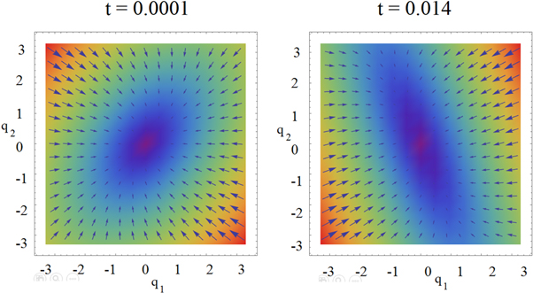
Figure 12. The total stochastic velocity at the start and the end of the quasi-stationary state. The state points  farthest from the center move at a greater velocity, while the points in the center are comparatively static. The velocities in the
  regions indicate the increase in probability at the central region.
Download figure:
Standard image High-resolution imageThe total stochastic velocity, shown in figure 12, is a two-dimensional field that plots the tendency of the state points  to move towards a region in the center, which intuitively coincides with the plot of the probability density. At the start of the reaction (
 ) it is mainly the points from the second and fourth quadrant that move at a greater velocity, contributing the most in keeping the saturation on the center. In contrast, when very close to the equilibrium (
 ) the roles have reversed, and it is now the first and third quadrants responsible of keeping the saturation in the center.
We calculate the curl of the total stochastic velocity to further explore this behavior, as shown in figure 13. From a geometrical viewpoint, the tendency of the field to rotate suggests that the averaged transitions performed by the state points,  within each region
  occur due to the lack of balance between the displacements
  which is something that is also reflected by the averaged
  This conduct causes the semi-axes of symmetry of the probability distribution to not remain static. The magnitude of this phenomenon diminishes with time, corresponding to the end of the quasi-stationary stage.

Figure 13. The curl of the total stochastic velocities is negative. We associate it with the tendency of the probability distribution to rotate clockwise during the quasi-stationary state.
Download figure:
Standard image High-resolution imageAbout the different terms of the entropy of the Michaelis-Menten model
Now we get back to the discussion about the entropy of the system that was left pending in expressions (36)–(38). The system under study is a laboratory experiment that progresses through time:
- At an initial stage, at a time interval we label as the enzyme and substrate molecules exist separate from one another.
- At an instant both substances get in contact with each other within a fluid that serves as a medium, at this point in time the reaction has not started. While the system is at where the reaction is yet to begin, the system can be considered as being in a state of thermodynamic equilibrium: It is for this reason that its entropy can be calculated using standard methods found in physical statistics.
- Let us suppose that the physical system is stirred to aid the start of the reaction. Once it starts, the time interval is which corresponds to the random process that has been discussed in previous sections. It is then than the entropy of fluctuations given in expression (26) makes itself apparent.


This section is dedicated to the study of entropy of the substrate and the enzyme-substrate complex. The working hypothesis is that the substrate and enzyme molecules are diluted in an aqueous medium, where they perform irregular motions. The physical system can be illustrated by the antibiotic penicillin playing the role of the substrate, and the beta-lactamase acting as the enzyme. The latter is used by bacteria to protect itself against the antibiotic.
At instant  when the reaction is about to start, we consider the substrate and enzyme molecules as if they are two ideal gasses with their respective entropy, which are originated by their degrees of freedom: translational, rotational and electronic. At instant
  the entropy of equilibrium, denoted as
  contains the terms shown in (114):

Where  is the translational entropy,
  is the entropy of mixing,
  is the vibrational entropy,
  is the rotational entropy, and
  is the electronic entropy. Save for
  we will calculate estimates for the values of the entropy of each contribution mentioned with the purpose of knowing an estimated value of
In this work we also add the fluctuation entropy,  for substrate and enzyme, which arises due to the dynamics of the Michaelis-Menten model. The resulting total entropy is given by (115):

It is compulsory to note the non-uniqueness of the definition of entropy in non-equilibrium systems. The definition of  is based in the one used in the theory of stochastic processes, but it should be made clear that there is no expression available for it that is generally accepted. In 2019, de Decker [34] demonstrated that, in the case of non-equilibrium systems, there are at least two definitions of entropy that, being both physically sound, differ in the time evolution of the production of entropy, even if both reproduce the same equilibrium state. However, even though the uniqueness of the time evolution is under contention, we consider appropriate the study of the special case of entropy in the processes that can be described by the Michaelis-Menten model.
Requirements for the decrease of entropy
The second law of thermodynamics establishes that, in the absence of external work being done on a system, entropy follows the inequality shown in (116):

Such that the equal sign is present once the state of equilibrium is reached.
Instead, entropy can diminish if energy is applied to a system through appropriate processes. We see that this is the case in enzymatic catalysis that are studied with the Michaelis-Menten model.
From the definition of Markov processes [34], it is clear that, in mathematical terms, the decrease of entropy through time is not forbidden. For a physical system with microscopic states numbered with  and its probability is denoted by
  its entropy can be expressed as seen in (117):

Its rate of change is given by (118):

From  results that
  Therefore, the inequality
  can be fulfilled if either of the conditions (119) or (120) are followed.


Calculating an estimation of the entropy of equilibrium
In this section we study the entropy in the time interval  up to equation (135). From that point on, the contribution of the entropy of fluctuations is added to the Michaelis-Menten model of the penicillin hydrolysis by the beta-lactamase. This is the case when the initial state of equilibrium is broken, then begins a process where the most important stage is the quasi-stationary state of the reaction, that reaches a state of equilibrium once the substrate has been exhausted.
The entropy of a system in statistical physics is calculated by  where
where  is the partition function. But as stated before, we will suppose that the system behaves like an ideal gas system. Therefore, for an ideal gas of
  particles of mass
  the expression for the entropy is given by:
Where  with
with  and
and  the number of substrate particles,
  the number of enzyme particles, and
  is the initial number of substrate and enzymes in the system. In this expression
  denotes the masses,
  is the mass of a substrate particle and
  is the mass of the enzyme particle.
Translation entropy
For the substrate, let us consider as an example the antibiotic rifampicin, which is part of the family of penicillin. The enzyme considered is the beta-lactamase. The data used to model these molecules is shown in table 4:
With a temperature of  the translation entropy of substrate and enzyme are given in (121) and (122), respectively.


Where  The total translation entropy is given by (123):

Mixing entropy
This contribution to the total entropy exists due to the existence of two gasses mixing inside a volume. The mixing entropy can be expressed as:

Where  and
and  The estimate of the mixing entropy is given by (124):

Vibrational entropy
Here we study the contribution to the entropy by the vibrations of enzyme and substrate molecules. We begin with the substrate.
Vibrational entropy of the substrate
The rifampicin molecule is relatively small when compared to that of the beta-lactamase. For this analysis we suppose that the molecules can be considered as oscillating nuclei that can be detected by IR spectroscopy, therefore we model the substrate as  independent harmonic oscillators, where
  denotes the frequencies, with
  The contribution to the entropy due to the vibrational degrees of freedom of the substrate can be calculated with:
This results in (125):

Ivashchenko [35] provides a set of wave numbers that, when transformed to frequencies, provide the following values:

For a temperature of  the vibrational entropy contribution of the substrate is shown in (126):

Vibrational entropy of the enzyme
The enzyme is a sizeable molecule, compared to the substrate, but its dimensions are still within the order of nanometers. For it we use the oscillatory theory of very small solids with the added correction necessary for such scales. The shape also plays an important role, but we will suppose it is a sphere of diameter between 3 to 7 nm, with a homogenously distributed mass.
Bu-Xuan Wang [36] argues that the theory of specific heats of Einstein can be applied to nanoparticles, thus, we use the partition function of solids [37] given as:
Using the hypothesis by Einstein of  with
with  being the Einstein frequency, and using the empirical adjustment parameter known as the Einstein temperature,
  the expression for the vibrational entropy of the enzyme can be obtained, as shown in (127):

Where  and
and 
According to E Gamsjäger [38],  for a temperature of
  the value of the vibrational entropy contribution of the enzyme is given in (128):

Entropy of rotation
A more precise treatment of the entropy of a large molecule, such as a protein or an enzyme, requires knowing its energy levels to be able to calculate its partition function. This has been considered a very complicated problem [39, 40], therefore we suggest the approach mentioned above, to treat it as a sphere of homogenously distributed mass.
The substrate, on the other hand, is by comparison a much smaller molecule. This can be modelled as if it was a nanometric ellipsoid with a homogeneously distributed mass  with its axes denoted by
  and
and  Taking its principal axes as the coordinated system, the tensor of inertia is diagonalized, and only three quantities are needed to describe it [41]:

The partition function resulting from the rotational degrees of freedom is denoted as such:
Which, defining  can be compacted as seen in (129):

The resulting entropy of rotation is of the form (130):

The underlying difference between the contribution from the substrate and from the enzyme is contained in the values of  and
and 
Entropy of rotation of the substrate
We suggest that, when the substate molecule rotates, the shape is similar to a spheroidal prolate. With this in consideration, it is possible to estimate its size based on the length of its  bonds (1.346 Å); therefore, its semiaxes would be:
With its mass given as:
The moments of inertia are of the form:
Since we have no information about its symmetry, we assume  which gives the result:

At a temperature of  the value of the estimation of the entropy of rotation contribution by the substrate is given by (132):

Entropy of rotation of the enzyme
For the estimation of the contribution to the entropy of rotation by the enzyme we consider the beta-lactamase, which will be modelled by a sphere of homogeneously distributed mass  Its measurements are presented below:
The resulting entropy of rotation for the enzyme is:

At a temperature of  the resulting entropy of rotation contribution by the enzyme is given by (134):

Entropy of equilibrium

Entropy of fluctuations
The entropy of fluctuation is made noticeable in the system once the interaction between enzyme and substrate begins. This moment in time will be labelled as 
According to the Michaelis-Menten model, it is enough to follow the substrate and the enzyme-substrate complex to have a proper understanding of the system. Under such consideration, we will see that there is a decrease in entropy.
The computer simulation was carried out with the reaction rates shown in table 5 [42] below. As shown in previous sections, the simulation displays three stages of the chemical reaction. Figure 14 shows the functions fitted to the means of  and
and  where, as before,
 and
and 
Table 5. Transitions rates used in the simulation of the penicillin hydrolysis catalyzed by beta-lactamase.

|

|

|

|

|

|

|

|

|
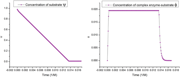
Figure 14. Time evolution of the substrate (left) and enzyme-substrate concentration (right).
Download figure:
Standard image High-resolution imageThe method used to calculate the means was the following:
- 1.The simulations were carried out number of times, with
- 2.Of the realizations, the one with the longest duration was selected. Its time was divided into intervals of equal width, with
- 3.The datapoints of the realizations that fell in each interval were averaged.


The curves fitted serve as confirmation of an initial stage when the substrate decreases rapidly as the enzyme-substrate complex increases drastically towards the second stage. During the second stage, almost all enzymes are in the enzyme-complex state, in other words, the concentration of free enzymes fluctuates near zero; this stage is what is called the stationary state in biochemistry. The third stage is reached when substrate is depleted, therefore the concentration of enzyme-substrate complex decreases exponentially. The time duration of each stage and the functions fitted for the substrate and enzyme-substrate complex during each of these can be seen in table 6, the curves are shown in figure 14.
Table 6. Time functions that parametrize the substrate and enzyme-substrate complex concentrations in 1st, 2nd and 3rd stage.
| Duration (s) |
 fit fit |
 fit fit | |
|---|---|---|---|
| 1st stage |

|

|

|
| 2nd stage |

|

|

|
| 3rd stage |

|

|

|
Equations (32) were solved numerically, then  was found using expression (36). The computer simulation allows us to find the entropy of fluctuations
  but, even though we consider the precision to not be enough to quantitively determine
  we can provide an approximation using the following initial conditions:

Adding the approximation of the entropy of fluctuations to the previously obtained entropy of equilibrium,  the result can be seen in figure 15. Some relevant values of the time evolution of
  are shown in table 7.
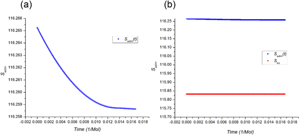
Figure 15. Left: Time evolution of the entropy of fluctuation. Right: Comparison between total entropy at  (start of the reaction), and entropy of equilibrium at
Download figure:
Standard image High-resolution image
Table 7. Numerical values of the entropy.  entropy of equilibrium.
  entropy of fluctuation during
 total entropy at the start of the reaction,
 Total entropy at
  (the end of the catalytic reaction).
  Decrease in entropy of fluctuation (
 ).
).

|

| |

|

| |

|

| |

|

| |

|

| |
The intriguing result seen in figure 15 and table 7 can be stated in two aspects:
- (1)It is clear that the net entropy of the reaction is greater than it was before the start of the reaction, therefore it is a spontaneous process.
- (2)The curve displayed in figure 15(a) shows a decrease in entropy, something that is only possible if there is an external energy source.
Before the reaction, the value of the total entropy is  Once the reaction starts (at
  ), the total entropy suffers a change, increasing a quantity of
  so the total entropy at that point is
  As the reaction takes place, the entropy decreases until the system reaches a state of equilibrium once the catalysis has finished (at
  ); the resulting decrease in entropy is
  so the total entropy at that point is
  It is important to note that the magnitude of the decrement in entropy,
  is lower than the increase in entropy due to the reaction taking place,
  in other words,
  According to the second law of thermodynamics, this decrement is evidence of the existence of work during the process of catalysis.
The value of  is approximately 1.52% of the initial entropy of fluctuations and it is 6.71% of the mixed entropy, this could be (as stated before) because the system is receiving energy in the form of work from an external source. A revision of the existing literature leads us to suggest that it comes from the vibrational degrees of freedom of the enzyme, which will be discussed below. For processes at constant volume, the fundamental equation of thermodynamics establishes:

The condition of  leads to the following inequality:
  Considering the quasi-stationary state as representative of the majority of the process of catalysis, then
  therefore the inequality takes the form of:

If  one must have
  so that this decrease in the entropy is consistent with results previously published: in enzyme catalysis happens that
  [43, 44]. Also, the negative value in this heat capacity is a condition to show that in enzyme catalysis there is an optimal temperature
  where the most efficient catalysis occurs.
The results from our computer simulation of a Michaelis-Menten system allows us to make a prediction that points towards the correct direction, since it reproduces the inequality of  for the entropy of fluctuations.
However, our model has a limitation in its quantitative aspect. According to Hobbs et al [43] and Arcus et al [44], the values of the heat capacity at constant pressure are within the range  If one is to take the right-hand value of the range, at
  with
with  converting to
  per particle, the resulting value of the change in entropy would be:
Furthermore, according to our results, the entropy of fluctuations per particle is:
This leads us to conclude that there is some aspect missing in this model.
Discussion
The Michaelis-Menten model partially captures the essence of the catalysis phenomenon in absence of cooperativity. It allows the prediction of the existence of a descent in the entropy of fluctuation, which corresponds with the experimental observation of the descent in the heat capacity at constant pressure,  during catalytic processes. Nonetheless, the difficulty of producing quantitatively precise results constitutes a limitation of the model. Although it has demonstrated its usefulness in processes that do not present cooperativity, its simplicity hinders it from capturing a wider range of phenomena specific to each reaction. For example, a revision of the mechanism of hydrolysis of penicillin by the beta-lactamase enzyme produced by bacillus cereus [45], pseudomonas aeruginosa, amongst others, show that the rupture and formation of chemical bonds in the process is more complicated than a catalysis reaction where only one enzyme-substrate complex participates as intermediary. This is a bigger problem than it may seem, as we argue below.
A. Holmberg [46] studied the practical difficulties that appear when estimating parameters in biological processes. He paid special attention to systems described by the Michaelis-Menten equation and proposed a sensibility function to deal with the lack of uniqueness in the results. The problem stems from different parameters reproducing the same experimental results. This indicates that there can be various physical processes that remain hidden within the parameters, which consequently gives way to a set of results being able to model the same substance. This leads one to think that, in the model, a compound as the enzyme-substrate complex can, in the real phenomenon, be two molecules even though in the Michaelis-Menten formulation appears only one.
J. Kim and J. Lee [47] pick up the topic of the difficulty faced when elaborating mathematical models to describe specific phenomena. They explore the case where differential equations with adjustable parameters, obtained from experimental data, are used with these purposes. Their suggestion is a set of mathematical tools to estimate the quality of the adjusted parameters. It is this complexity in the analysis that clearly displays the issues confronted when modelling from experimental data.
A similar problem appears in systems modelled with the Langevin equation and the Fokker-Planck equation. In one dimension both formulations are equivalent, but in two or more dimension, two Langevin equations corresponding to two different physical systems lead to the same Fokker-Planck equation.
In conclusion, while it is praiseworthy that the Michaelis-Menten model sheds light on the qualitative understanding of the role of the entropy in the catalytical process, its quantitative prediction is a much more complicated field of study.
Possible repercussions in pharmaceutical technology
In recent years, there have been developments in the use of nanostructures as drug carriers [48]. In the design of these processes, it is often suggested that drug carriers could accumulate in specific sites where they would then release their load, thus increasing the efficiency of the medicine [49], as well as a reducing its toxic effects in the patient undergoing treatment. If one supposes that these nanocages have a specific size, for example a diameter of  it is possible to estimate the capacity of each drug carrier: If
  and the carrier is spherical, its effective volume would be
  now, if the volume occupied by a molecule of a drug like amoxicillin is that of a square prism of sizes
  [50], giving the amoxicillin molecule an effective volume of
  If the volume within the nanocage is occupied by this drug, the maximum quantity of molecules it could carry would be
  However, if the nanocage carries an aqueous solution of amoxicillin and clavulanic acid, in proportions similar to those found in injectable solutions
  [51], the antibiotic occupies approximately only 5% of the space, meaning that there are of the order of 1434 molecules of antibiotic in the load. This means that purely deterministic models would only offer a partial understanding of the system.
With regard to stochastic mathematical models used to describe the transport and release of drugs in living tissue, these tend to focus on the concentration of the drug over time [52] and are based on basic equations, like the diffusion law of Fick in different geometries. These can also incorporate other relevant details, such as local tissue inflammation and degradation of the polymer drug carrier.
With this in mind, we believe that the inclusion of other thermodynamic magnitudes, beside particle concentration, to the description of the process would prove useful. One such magnitude could be the elastic properties of the beta-lactamase molecule during the hydrolyzation of the antibiotic.
The usual approach for studying molecular vibrations consist in supposing that the force constants between atoms are independent of the temperature of the medium. This idea is introduced in statistical physics through the occupation of energy levels, without considering the possibility that the vibration frequency of the particles that give form to the molecule depend on the temperature. In contrast with this methodology, Kolesov [53] considers the changes in temperature as a means to fine tune atomic bond length and atomic interaction. He suggests that  is the vibration frequency at a temperature of
  and for increasing values of
  the relation
  is followed.
If the approach by Kolesov is true, it could open the way to new processes and techniques that would allow the local manipulation of temperature to interfere with the normal vibration modes of the molecule, aiding in the transfer of energy towards the process of catalysis.
Conclusions
The treatment by Bartholomay was reformulated by van Kampen through his omega expansion. The  state space, for substrate and enzyme-substrate complex molecules, respectively, was split in two spaces:
- A state space for the macroscopic concentrations. This reproduces the dynamics of the Michaelis-Menten that are found in textbooks.
- A state space for the fluctuations, known as the fluctuation space. It is studied through time dependent Ornstein-Uhlenbeck processes, adding to the understanding of the enzymatic reaction kinetics that can be described by the Michaelis-Menten model.
A simulation based in the Gillespie algorithm allows a clear configuration of the quasi-stationary state under study. The theory and the simulation help us demonstrate that the probability density in the fluctuation space is a gaussian function that rotates clockwise. The auto-correlation functions tend to a constant at the end of this stage.
The formalism of stochastic velocities proves useful when studying the fluctuations described by gaussian probability densities. The curl of the total stochastic velocity is negative, explaining the tendency of the probability density to rotate. It is this tendency to rotate that explains the lack of detailed balance during the quasi-stationary state
The estimation of the entropy displays a sudden increase in its value once the reaction starts, and a subsequent minor descent as it progresses. Here two important aspects of the process combine:
- 1.The increase in entropy indicates a spontaneous chemical reaction.
- 2.Its descent supports the existence of a rearrangement process during catalysis, as well as the presence of work being performed on the system.
We propose that the source of this energy are the normal vibration modes of the enzyme inside a medium at a given temperature. This also backs up the negative sign in the change of heat capacity at constant pressure,  that has been found by other researchers, who consider it a fundamental part for the existence of an optimal temperature in the efficiency efficacy of the catalytic ability of enzymes. The Michaelis-Menten model has been notably successful in this aspect, but it shows an important limitation when quantitatively predicting the magnitude of the descent of
Data availability statement
The data that support the findings of this study are available upon reasonable request from the authors.