


Abstract
We propose a new scheme to prepare macroscopic entanglement between two rotating mirrors using dissipative atomic reservoir in a double-Laguerre–Gaussian-cavity system. The two-level atomic system driven by a strong field, acts as a single pathway of Bogoliubov dissipation to push the two original cavity modes into the desirable entangled state under the near-resonant conditions. Successively, the photon–photon entanglement can be transferred to mirror–mirror entanglement through the exchange of orbital angular momentum. In essence, the macroscopic entanglement is originated from the dissipative atomic reservoir rather than the radiation torque, thereby it is usually robust against environmental noises. The present scheme provides a feasible way to realize stable entanglement between spatially separated mirrors with high capacity, which may find potential applications in remote quantum communications.
Export citation and abstract BibTeX RIS

Original content from this work may be used under the terms of the Creative Commons Attribution 4.0 license. Any further distribution of this work must maintain attribution to the author(s) and the title of the work, journal citation and DOI.
1. Introduction
In recent years, the interaction between structured light beams and matter has been paid continuous attention in quantum optics and quantum information. Particularly, the Laguerre–Gaussian (LG) beam, as a typical type of structured light, can be obtained by solving the paraxial wave equation in cylindrical coordinates, possessing a helical wavefront and a doughnut-shaped intensity distribution with a hollow at the beam center [1, 2]. The LG beam usually carries an orbital angular momentum (OAM) of  per photon with its phase of
  , where l is topological charge value and φ represents azimuthal angle [3]. In experiment, the typical methods to generate LG light are spatial light modulators [4, 5], spiral phase plate or mirror [6, 7] and computer-generated holograms [8, 9]. It is demonstrated that the topological charge value l can reach as high as 1000 by using the spiral phase plate [10]. Interestingly, the LG beams can exert a torque on objects due to the exchange of OAM [11–13], with which it is possible to trap and cool the rotational mirrors [14]. So far, a large number of quantum optics phenomena have been reported based on the interaction of LG light with matter, including the vortex light information storage [15], quantum memory [16], spatially dependent electromagnetically induced transparency [17], transfer of optical vortices via the multi-wave mixing [18–21], optomechanical induced transparency [22], ground-state cooling [23], the detection of OAM [24], the generation of higher order sideband [25, 26], and the high-dimensional quantum entanglement [27–34] etc.
On the other hand, the macroscopic entanglement is of great importance both in verifying the fundamental quantum theory [35] and realizing realistic applications such as remote quantum communication, reliable quantum computation, precision measurement and quantum sensing [36, 37] etc. In experiment, the entanglement between two macroscopic objects is demonstrated by engineering the dissipation with laser and magnetic fields [38]. The mechanical resonator at the micrometer scale, an ideal candidate for investigating macroscopic entanglement, has attracted much attention in last years because it locates at the interface of the quantum-to-classical transition [39–44]. It is explored that the macroscopic oscillators can be entangled by using the radiation pressure, behind which both the parametric interaction and beam splitter interaction are hidden [45]. Successively, various literatures focus on the methods to entangle two massive, movable cavity mirrors at steady state [46–49]. As a profitable model, the bipartite and multipartite entanglement between mirrors and cavity modes are also acquired under the effect of radiation pressure force [50, 51]. Interestingly, it provides a useful way to control the macroscopic entanglement by atomic coherence effects [52–56], in which the parametric interaction between mechanical oscillators is established by the coherence-controlled evolution processes. A lot of recent studies show that the hybrid quantum systems have developed an extensive platform to generate macroscopic entanglement between distant objects [57–60], which may find potential applications in remote quantum communications.
Notably, in a rotational optomechanical system, Bhattacharya opens up fascinating possibilities, in their pioneering works, to entangle a LG cavity mode and a rotating mirror [61], or generate entanglement between the rovibrational modes of a macroscopic mirror using radiation pressure [62]. Motivated by this device, Chen et al report the macroscopic entanglement between two rotating mirrors through the exchange of OAM with the same LG cavity [63]. Later, by placing a yttrium iron garnet (YIG) sphere into the LG cavity, the tripartite entanglement are generated between cavity mode, mirror and magnon [64]. While the YIG sphere is replaced by a two-level atomic ensemble, the cavity–mirror entanglement and quantum coherence are enhanced by choosing suitable parameters [65], which is attributed to the fact that the effective coupling of the parametric interaction is enhanced by injecting the atoms. Nevertheless, the quantum coherence would be spoiled when the large detuning limit is not satisfied. In addition, they point out that the quantum coherence are also significantly suppressed by the large atomic decay.
In this paper, we present a different way to establish macroscopic entanglement between two spatially separate rotating mirror via a single pathway of Bogoliubov dissipation. The main results we find in the present scheme are listed as follows. First, in dressed-state picture, it is seen that the two original modes constitute a pair of Bogoliubov modes, one of which mediates into the interaction while the other 'dark mode' is decoupled with the system. When the dissipation process is dominant over the amplification process, the Bogoliubov mode would evolve into a squeezed vacuum state, causing the generation of entanglement. This entangled state is successively transferred to two rotating mirrors via the beam splitter interaction. Obviously, the macroscopic entanglement is essentially originated from dissipation rather than radiation torque. Second, we find that the optimal macroscopic entanglement can be obtained when the driving field is nearly resonant with the atomic transition. There exists two extreme cases where the entanglement is vanished. At the exact resonant condition, the entanglement disappears since the dissipation rate is negligible when the dressed-state populations are identical. For the large detuning cases, the entanglement is also significantly suppressed due to the reduction squeezing parameter. Therefore, the best entanglement is obtained at an appropriate value of driving detuning. Third, we note that the macroscopic entanglement can be obtained when the damping rates of the atoms are much larger than the cavity losses, i.e.  . As a result, the atomic system can be viewed as a reservoir and the treatment of adiabatically eliminating atomic variables is valid. We extract the atomic contribution of the dissipative reservoir effects clearly and the quantum noises from atoms are included to calculate the quantum entanglement. Our results explore that the atomic damping rates have positive effects on macroscopic entanglement, which is completely different from the schemes in [65]. Finally, comparing with previous schemes [61–65], the macroscopic entanglement can be simply controlled by the strength and detuning of the driving field on atoms, which may provide conveniences for experimental implement.
The remaining part of the present paper is organized as follows. In section 2, we describe the system model of the double-Laguerre–Gaussian-cavity (DLGC) system. The master equation and Heisenberg–Langevin equations for the cavity modes and rotating mirrors are derived. In section 3 we present the physical mechanisms and discuss the numerical results of the remote mirror–mirror entanglement with two different methods. Finally, the conclusion is given in section 4.
2. Model and equations
The rotational DLGC system under consideration is presented in figure 1(a), in which the system consists of two fixed mirrors (FM ) and two rotational mirrors (RM
 ). We consider that a two-level atomic ensemble is placed at the cross site of the two cavities. The RM mirrors are mounted on the support points S
 and can rotate around the axis Z
 , respectively. Without loss of generality, we assume that the fixed mirrors FM
 are partially transparent while RM
 have perfect reflection. When the LG beams G
 with 0 charge are incident on FM
 , we only consider the transmitted beams with unchanged 0 charge since the reflected components do not interact with the atomic ensemble. The two 0 charge beams reflected from the RM
 can get charged to
  . It has been explored in experiment that LG beams can exert a torque on microscopic particles, in which the optical vortices are generated [13]. In addition, Bhattacharya and Meystre et al use OAM transfer from a LG beam to trap and cool the rotational motion of a macroscopic mirror made of a perfectly reflecting spiral phase element [14]. Assuming both RMs have the same mass m and radius r0, their moments of inertia about the axis Z
 passing through the center are
  . The RM
 oscillate like two pendulums with angular frequencies
  . Notably, the RM
 act as two harmonic oscillators for the angular deviations
  and they have the equilibrium position
  . Apart from the internal spin angular moment (
 ), photons in LG beams carry integral OAM numbers
  , respectively [2]. Therefore, when the LG beams are incident on the cavity, they can transfer torques
 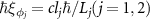 per photon to the RM
 , in which c represents the velocity of light and
  are the length of the two cavities. Then the mechanical effects of the LG beams interacting with the macroscopic rotating mirrors should be considered. The Hamiltonians of the DLGC system plus the atomic ensemble are written as

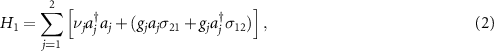

wherein H0 represents the system Hamiltonian for the two-level atoms driven by a strong field with frequency ω0 and Rabi frequency Ω. The atomic transition frequency is denoted by ω21.  are the projection operators of N independent atoms for l = m and the flip operators for l ≠ m. H1 describes the free Hamiltonian of the two cavity modes plus the interaction Hamiltonian between the atoms and cavity modes with coupling constants
  . aj
(
. aj
( ) are the annihilation (creation) operators for the two cavity modes with the frequencies νj
. H2 denotes the free Hamiltonians of the two rotational cavity mirrors, the interaction between the cavity modes and two rotating mirrors, the driving Hamiltonian to the cavity modes by the external laser fields with frequencies
) are the annihilation (creation) operators for the two cavity modes with the frequencies νj
. H2 denotes the free Hamiltonians of the two rotational cavity mirrors, the interaction between the cavity modes and two rotating mirrors, the driving Hamiltonian to the cavity modes by the external laser fields with frequencies  and the amplitudes of
  , wherein κj
are the cavity damping rates and Pj
input power of the laser.
, wherein κj
are the cavity damping rates and Pj
input power of the laser.  are the angular momentum of RM about the axis with the commutation relation [
 , φk
] =
, φk
] =  . According to [14], we can define
in which the annihilation and creation operators for the rotating mirrors are denoted by bj
and  , respectively. Substituting the above expression into equation (3), making a unitary transform with
  exp
exp and
and  , we can rewrite the Hamiltonian H0 and H1 as


where  ,
,  ,
,  are cavity detunings, atomic detunings and driving detunings, respectively. The coupling parameters Gj
are defined as
are cavity detunings, atomic detunings and driving detunings, respectively. The coupling parameters Gj
are defined as  .
.
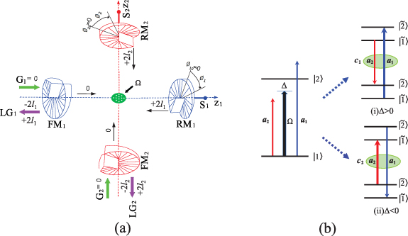
Figure 1. (a) Schematic diagram of DLGC system. The system consists of two fixed mirrors (FM ) and two rotating mirrors (RM
 ). A two-level atomic ensemble driven by strong field Ω is placed at the intersection of the two cavities. The RM mirrors are mounted on the support points S
 and can rotate around the axis Z
 , respectively. We assume that the fixed mirrors FM
 are partially transparent while RM
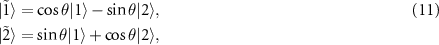
 have perfect reflection. (b) The energy level structure of the two-level atomic system, in which Ω is the Rabi frequency and Δ represents the atomic detuning. The two cavity fields denoted by annihilation operators
  couple to the common atomic transition with different cavity detunings. For
  , the original modes
  are resonant with the Rabi sidebands and they constitute a Bogoliubov mode c1 to mediate into the interaction. In the other case of
  , c1 is replaced by the other Bogoliubov mode c2 to interact with the atomic system.
Download figure:
Standard image High-resolution imageThe atomic relaxation, the cavity losses and the intrinsic damping rates of rotating mirrors are taken the forms as


To obtain the reduced master equation of cavity modes, as proposed in [66], we resort to the dressed atomic picture by diagonalizing the Hamiltonian  under the conditions of
  . The dressed atomic states are expressed in terms of bare states as [67]
in which 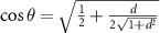 and
and 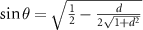 with normalized detuning
  . The dressed states
  and
and  have their eigenvalues
  with
with  , respectively. Now the system Hamiltonian of
  is rewritten in the dressed-state picture as
  . By transforming the bare atomic relaxation term (8) into the dressed-state picture and neglecting the quantized mods temporarily, the steady-state populations of the dressed states
  are obtained as

Clearly, for  , we have
  and
and  , namely, the populations of the two dressed states are identical at the exact resonant condition. For
  , we have
  (or
(or  when
when  (or
(or  . The equilibrium is broken and then the dissipative atomic reservoir effect is possible [68]. Making a further unitary transformation with
  on the Hamiltonian
  , the effective Hamiltonian is derived as

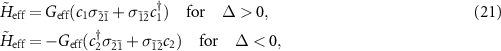
in which we take the conditions of  , i.e. the cavities are tuned to be resonant with the Rabi sidebands. If the cavity detunings are tuned to be comparable to or larger than the level spacing
  , the effective Hamiltonian is no longer valid. Under the good-cavity limit of
  (
( ), the atomic variable can be adiabatically eliminated using the standard quantum optics techniques [69, 70]

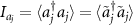
Finally, the reduced master equation of the cavity modes takes the form
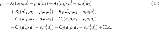
where the parameters are 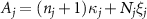 ,
,  , and
, and  (
( ) with the coefficients
  ,
,  ,
,  . Here nj
represent the mean thermal photon number of the cavities.
. Here nj
represent the mean thermal photon number of the cavities.
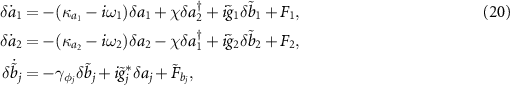
In present scheme, we focus on investigating macroscopic entanglement between two rotating mirrors. To do so, we make use of reduced master equation (15) and the Hamiltonian  to obtain the dynamics equation as
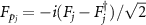
For simplicity, we define  ,
,  ,
,  ,
,  . Fj
are noise operators including the cavity losses and the atomic contribution part.
. Fj
are noise operators including the cavity losses and the atomic contribution part.  represent the mechanical noise operators coupling to the rotating mirrors from the thermal environment. Without loss of generality, we have vanishing mean
  and the nonzero second order correlation terms
 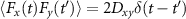 as
as
wherein ![$n_{\phi_{j}} = [\textrm{exp}\frac{\hbar\omega_{\phi_{j}}}{/k_\mathrm{B}T_{j}}-1]^{-1}$](https://content.cld.iop.org/journals/1367-2630/24/12/123044/revision2/njpacae3cieqn94.gif) is the mean occupation number,
is the mean occupation number,  is the Boltzmann constant and Tj
the environmental temperature of the mechanical resonator.
is the Boltzmann constant and Tj
the environmental temperature of the mechanical resonator.
According to equation (16), by defining  , we can neglect the the highly oscillating terms for
  and then the steady-state solutions for
  and
and  are derived as
The equation for the intracavity mean photon numbers is given by

in which we define  ,
,  . It is clear that the two rotating mirrors will exhibit optical bistable behavior and experience strong nonlinearities, which can be controlled by the detuning and strength of the driving field on atoms.
To explore the macroscopic entanglement between two rotating mirrors, we can linearize the equation (16) around the semiclassical state corresponding to a working point in the stable range, i.e.  . The steady state solutions
  are given in equation (18) and
  represents the quantum fluctuation around the mean value. Furthermore, we introduce the slowly varying fluctuation operators
  and
and  . By dropping the high-frequency oscillating terms
 ![$\exp[-i(\delta_{1}+\delta_{2})t]$](https://content.cld.iop.org/journals/1367-2630/24/12/123044/revision2/njpacae3cieqn107.gif) at
at  , the corresponding linear quantum Langevin equations for the quantum fluctuations are obtained as
wherein 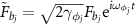 ,
,  . Then the quantum entanglement between the two mirrors can be calculated and discussed according to the above equations, which will be presented in the following section.
3. Analysis and discussion
In this section, we would like to elucidate the mechanism for the generation of rotational optomechanical entanglement. Next, the numerical results of mirror–mirror entanglement are presented by nonadiabatical eliminating and adiabatical eliminating of cavities, respectively. The possible experimental parameters are briefly discussed in the last subsection.
3.1. Physical mechanism analysis
3.1.1. Dissipation of cavity fields in light of Bogoliubov modes
In order to describe the internal mechanisms for the generation of quantum entanglement more clearly, we define a pair of Bogoliubov modes in equation (13) for the cavity fields:  ,
, 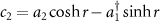 with the squeezing parameter
  for
for  and
and  for
for  . The interaction between the dressed atoms and the Bogoliubov mode is shown in figure 1(b). Correspondingly, the system Hamiltonian of equation (13) is simply rewritten as
where the effective coupling constant 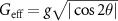 by assuming
  . Note that only the collective mode c1 (or c2) mediates into the interaction while the other mode c2 (or c1) is decoupled with the system for the two cases. This is termed as a single pathway of Bogoliubov dissipation, which can lead to the occurrence of quantum entanglement [66, 68]. Under the adiabatic elimination conditions of
  , we can obtain the atomic contribution part of the reduced master equation for the Bogoliubov mode
  as
as

in which 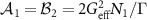 and
and 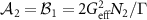 with
with  . It is seen that the
  terms represent the dissipation and the
  terms denote the excitation of Bogouliubov modes, respectively. When dissipation rate
  , the Bogoliubov mode c1 (or c2) will evolve into the squeezed vacuum state while the other mode c2 (or c1) is decoupled with the system. Generally, the larger the dissipation rate is, the stronger the entanglement will be. For
  , we have
  and
and  , leading to the absence of quantum entanglement, which is verified by the following numerical calculations. However, when the normalized detuning d deviates slightly away from the resonant conditions, we have
  in the positive (
 ) and negative frequency regions (
 ) due to
  , thus resulting in the appearance of entanglement. For example, at d = 0.3, we have
  ,
,  and
and  , meaning that the adiabatical elimination of atomic variables and the single-pathway dissipation of Bogoliubov are valid. On the other hand, the entanglement is simultaneously determined by the squeezing parameter r. When d is increased, the squeezing parameter r is inversely decreased accompanying by the increasing of the dissipation rate
  . For example, the squeezing parameter (
 =
=  ) is r = 1.15 at d = 0.1, r = 0.41 at d = 0.5, and r = 0.17 at d = 1. As a consequence, the best entanglement appears at the near-resonant conditions when the dissipation rate and the squeezing parameter r have a compatible value.
3.1.2. Entangled state transfer from cavity fields to rotating mirrors
Next, we would like to clarify the frequency arrangement of the present system. As shown in figure 2(a), on the one hand, the cavity fields  are tuned to be resonant with the sidebands, i.e.
  . For the cavity detunings
  , we have
  . On the other hand, it is seen that the frequencies of the rotating mirrors
  and the frequencies of driving fields on cavities
  satisfy the relations of
  . Due to the driving detunings
  , we have the relations of
  , giving rise to that the high-frequency oscillating terms
 ![$\textrm{exp}[-i(\delta_{1}+\delta_{2})]$](https://content.cld.iop.org/journals/1367-2630/24/12/123044/revision2/njpacae3cieqn158.gif) in equation (20) should be dropped. Obviously, these terms with the form of
in equation (20) should be dropped. Obviously, these terms with the form of  describing parametric amplification are absent while the terms of
 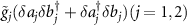 being responsible for quantum state transfer are existent [71]. In addition, as shown in figure 2(b), the internal physical mechanisms for the generation of macroscopic entanglement are depicted in detail. For
  , two original modes
  constitute a pair of collective modes
  , in which the 'bright mode' c1 would dissipate into the atomic reservoir for
  while the other 'dark mode' c2 (not shown) is decoupled with the system. As a result, the bipartite photon–photon entanglement is essentially established by the atomic reservoir effects and then it is transferred to two macroscopic rotating mirrors at
  via the two transfer processes
  . Finally, it is worthwhile to point out that the present system is completely different from the previous schemes proposed in [65]. In their works, the two-level atomic ensemble or magnon is placed into the cavity to enhance the cavity–mirror entanglement or to realize the tripartite entanglement based on the parametric interaction.
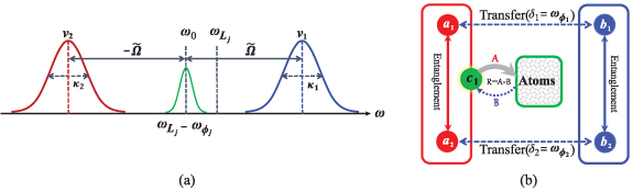
Figure 2. (a) The demonstration of frequency arrangement for the cavity modes, rotating mirrors and driving fields. It is seen that the frequencies for the drive fields satisfy the relations of  . The two cavity modes are tuned to be resonant with the red sideband and blue sideband
  , respectively. (b) Schematic demonstration for the rotating mirror-mirror entanglement in the case of
  . The two original modes
  constitute a pair of Bogoliubov modes
  to mediate into the interaction with dressed atoms. For
  , the collective mode c1 is replaced by c2 as shown in equation (21). When the dissipation coefficient is larger than the gain coefficient,
  , the collective mode c1 will evolve into a squeezed vacuum state while the mode c2 (not shown) is decoupled with the system, giving rise to the entanglement between two modes
  . Successively, the entangled state is transferred to the macroscopic mirrors via transfer and cooling processes at
  .
.
Download figure:
Standard image High-resolution image3.2. Rotating mirror–mirror entanglement without adiabatic elimination of cavities
In the first of place, we assume that the cavity modes are not adiabatically eliminated. To numerically calculate the quantum correlations between the two rotating mirrors, two pairs of quadrature operators are defined as  ,
,  ,
,  ,
,  . Then we can write the dynamical equations of quantum fluctuations in a concise form

where  ,
,  . The corresponding composite noise operators are written as
  ,
,  ,
,  ,
,  . The drift matrix M takes the form
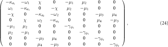
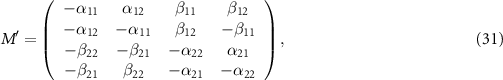
where in  ,
,  ,
,  ,
,  . Generally, the system would be stable if the real parts of all eigenvalues of M are negative, which can be judged based on numerical calculation in the present scheme [72]. Throughout this paper, we always guarantee that the system is stable via choosing appropriate system parameters. When the stability conditions are fulfilled, the steady-state Lyapunov equation is given by [50]

in which D denotes the diffusion matrix and V is a  covariance matrix (CM) with the matrix elements of
 ![$V_{ij} = \frac{1}{2}[\langle u_{i}(\infty)u_{j}(\infty)\rangle+\langle u_{j}(\infty)u_{i}(\infty)\rangle]$](https://content.cld.iop.org/journals/1367-2630/24/12/123044/revision2/njpacae3cieqn182.gif) . The CM of two modes is taken the form as
. The CM of two modes is taken the form as

wherein the matrix V1, V2 and V3 are the  submatrices. The diffusion matrix D are defined as
  and the nonzero diffusion coefficients are
  ,
,  ,
,  ,
,  ,
, 
 .
.
Once the CM of the system is achieved, one can calculate the degree of the mirror-mirror entanglement. We adopt a reliable logarithmic negativity criterion to study continuous variable quantum entanglement for Gaussian states [73, 74]. The definition of  is given by

where ![$\Lambda = 2^{-1/2} [\Sigma - \sqrt{\Sigma^2 - 4\det{V}}]^{1/2}$](https://content.cld.iop.org/journals/1367-2630/24/12/123044/revision2/njpacae3cieqn200.gif) with
with  .
.
In the following numerical calculations, the possible experimental parameters are listed in table 1 as proposed in [14, 61, 62]. In figure 3, the evolution of logarithmic negativity  is plotted versus the normalized detuning d and quality factor Q of cavities by choosing the OAM as
  . The angular frequencies of rotating mirrors are
  MHz and
  MHz. The cavity-atom coupling constants are always set as
  MHz. It is found that the entanglement first increases to a maximal value and then decreases slowly to zero in the positive frequency region. At this time, the entanglement disappears in the negative frequency domain because the stability condition is not satisfied when
  . On the contrary, the stability condition would be satisfied in the region of d < 0 for
  . Specially, at d = 0, as shown in equation (22), the gain coefficients
  are equal to the absorption coefficients
  for
for  , yielding the disappearance of mirror–mirror entanglement together with the single-pathway dissipation. Differently, with the increasing of normalized detuning d, the best entanglement happens at an appropriate value of d. Besides, we notice that the entanglement is remarkably enhanced and the entanglement region becomes wide with high quality factor Q.
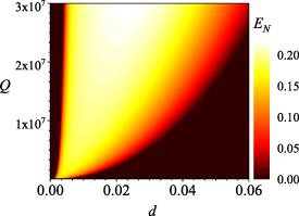
Figure 3. The logarithmic negativity  is plotted as a function of the normalized detuning d and the cavity quality factor Q for
  ,
,  MHz and
  MHz. The other parameters are chosen as those in table 1.
Download figure:
Standard image High-resolution imageIn figure 4, the logarithmic negativity  is plotted as a function of the angular frequency ratio of
  for two cases: (a)
  ; (b)
; (b)  by choosing different quality factor
  (solid line),
  (dashed line),
  (dotted line), respectively. The normalized detuning d is chosen as d = 0.012 and the input powers are
  mW. From these figures, it is found that the variation trend of
  is similar to that in figure 3. Notably, at
  , the entanglement vanishes for
  while occurs for
  , which can be attributed to that there is no exchange of total orbital angular moment between the cavity modes and rotating mirrors since the system is totally symmetrical [63]. Such a balance is broken for
  , leading to the generation of quantum entanglement at
  .
.
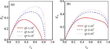
Figure 4. The logarithmic negativity  is plotted as a function of the angular frequency ratio rφ
for two cases: (a)
is plotted as a function of the angular frequency ratio rφ
for two cases: (a) ; (b)
; (b)  ; We choose the parameters as
  MHz, d = 0.012,
  mW,
mW,  (solid line),
  (dashed line),
  (dotted line), respectively. The other parameters are chosen as those in table 1.
Download figure:
Standard image High-resolution imageNext, we plot the entanglement evolution of  versus the input power
  . The other parameters are chosen as
  ,
,  MHz,
MHz,  MHz. In figure 5(a), logarithmic negativity
  is plotted by choosing different quality factor
  (solid line),
  (dashed line),
  (dotted line) and the influence of the rotating mirror masses on quantum entanglement is shown in figure 5(b) by choosing
  ng (solid line), 75 ng (dashed line), 100 ng (dotted line) for
  , respectively. As seen from figure 5(a), we have
  mW at
mW at  ,
,  mW at
mW at  and
and  mW at
mW at  . Obviously, the larger the quality factor is, the smaller the threshold power Pth will be. From figure 5(b), the threshold power Pth is changed from 136 mW, 205 mW to 271 mW when the mirror masses are increased from 50 ng to
  ng, demonstrating that the macroscopic quantum effects are modified by the system parameters including mirror mass m, cavity length L and the mirror radius r0 etc.

Figure 5. (a) The dependence of logarithmic negativity  on the input power
  by choosing different quality factor
  (solid line);
  (dashed line);
  (dotted line). (b) The evolution of logarithmic negativity
  versus input power by choosing different masses of rotating mirrors
  ng (solid line), 75 ng (dashed line), 100 ng (dotted line). The OAM is chosen as
  and the other parameters are the same as those in table 1.
Download figure:
Standard image High-resolution imageThe density plot of logarithmic negativity  versus the OAM l and the normalized detuning d is shown in figure 6(a) and the two-dimensional curves are plotted in figure 6(b) by setting
  . The parameters are chosen as
  MHz,
MHz,  MHz,
MHz,  MHz,
MHz,  and the mirror masses are chosen as
  ng. As shown in figure 6(a), when the absolute value of
  is increased, the entanglement appears and the region for
  becomes wide. To show this characteristic more clearly, the two-dimensional curves of the logarithmic negativity
  are plotted in figure 6(b) by choosing different normalized detuning d. It is seen that the best entanglement appears at an appropriate value of l, which can be used to detect topological charge value via the measurement of quantum entanglement.
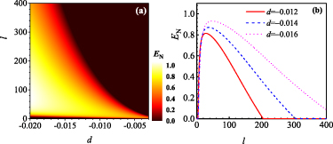
Figure 6. The logarithmic negativity  is plotted as a function of the OAM
  and the normalized detuning d. The other parameters are chosen as those in table 1.
Download figure:
Standard image High-resolution imageFigure 7 shows the evolution of logarithmic negativity  as a function of
  by choosing different OAM numbers of l for
  . It is clear that the good entanglement is obtained under the conditions of
  . With the increasing of
  , the values of logarithmic negativity
  are monotonously decreased to zero at a specific value of
  . By changing l from 200 to 500, the entanglement disappears at
  , 0.088, 0.05, 0.03, respectively. When the cavity losses are comparable to the atomic damping rates, the entanglement would be vanished, which is different from the results presented in [65]. What's more, the effects of thermal noise on quantum entanglement are also discussed in figure 8. The parameters are the same as those in figure 6(b) except for
  . As shown in figures 8(a) and (b), we find that the entanglement is relatively robust against environmental noise although it becomes worse as the thermal occupation numbers of
  and
and  increase.
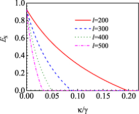
Figure 7. The evolution of logarithmic negativity  versus
  by choosing different OAM numbers l = 200 (solid line), 300 (dashed line), 400 (dotted line), 500 (dash dotted line) with
  , the normalized detuning
  , m = 10 ng,
  ,
,  µm. The other parameters are chosen as those in table 1.
Download figure:
Standard image High-resolution image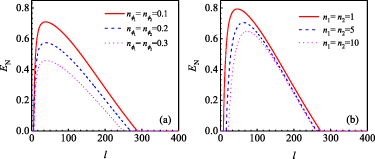
Figure 8. (a) The evolution of logarithmic negativity  versus the orbital momentum angular l by choosing different phonon numbers of
  in (a) and different thermal photon numbers of n in (b). The other parameters are the same as those in figure 6(b).
Download figure:
Standard image High-resolution image3.3. Rotating mirror–mirror entanglement with adiabatic elimination of cavities
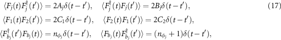
Usually, the damping rates of the rotating mirrors are much smaller than the cavity losses, i.e.  . Then we derive the fluctuations dynamical equations for the two rotating mirrors by adiabatically eliminating cavities as
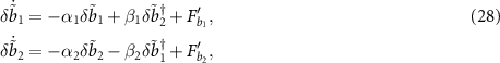
where the parameters  ,
,  ,
,  with
with  ,
,  . The noise operators are given by
in which we have the coefficients  ,
,  ,
,  and
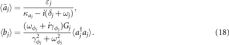
and  . From the equation (28), it is seen that the parametric interaction is hidden behind the effective Hamiltonian of the two rotating mirrors. This can be used to explain the physical origin of the remote mirror–mirror entanglement. It is worthwhile to point out that the parametric interaction arises from the two-photon process in dissipative atomic reservoir effects rather than the exchange of OAM. Interestingly, as show in equation (29), we find that the dissipation effects of the present system are determined by the following four factors: the atomic decay rate γ, the thermal noise of the mechanical oscillators
  , the cavity dissipation κj
and the coherent-controlled dissipative atomic reservoir effect. Being different from the previous work [52–54], we find that the dissipative atomic reservoir plays an important role in generating rotating mirror–mirror entanglement, which may find potential applications in remote quantum communications.
, the cavity dissipation κj
and the coherent-controlled dissipative atomic reservoir effect. Being different from the previous work [52–54], we find that the dissipative atomic reservoir plays an important role in generating rotating mirror–mirror entanglement, which may find potential applications in remote quantum communications.
In order to verify the validity of the adiabatic elimination approach, we follow the same procedure as in the preceding subsection to investigate the mirror–mirror entanglement with the same criterion. The dynamical equations of the quantum fluctuations of the rotating mirrors are written in a concise form as

in which the column vectors  ,
,  and the drift matrix Mʹ is derived as
where  ,
,  ,
,  ,
,  ,
,  ,
,  ,
,  and
and  . The quadrature noise operators are defined as
 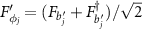 and
and 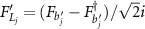 . According to Lyapunov equation, we can calculate the quantum correlations between two mirrors numerically. Notably, the nonzero diffusion coefficients can be calculated based on equation (29). For simplicity, the cumbersome expression of the diffusion matrix is not presented here.
In figure 9, we plot the logarithmic negativity  versus the input power and OAM for adiabatical and nonadiabatical elimination cases. The parameters are chosen as
  MHz,
MHz,  MHz,
MHz,  ,
,  MHz,
MHz,  ng,
ng,  ,
,  MHz and the other parameters are the same as those in table 1. It is seen that the results of adiabatical elimination cases are in well agreement with the nonadiabatical elimination cases when the condition of
  is satisfied, indicating that both methods are valid for calculating the quantum entanglement.

Figure 9. (a) Plots of logarithmic negativity  versus input power P with
  . (b) The evolution of logarithmic negativity EN
versus the OAM l1 = l2 = l with
. (b) The evolution of logarithmic negativity EN
versus the OAM l1 = l2 = l with  mW for adiabatical elimination (solid line) and nonadiabatical elimination (dashed line) cases. The parameters are chosen as
  MHz,
MHz,  MHz,
MHz,  ,
,  MHz,
MHz,  ng,
ng,  ,
,  and the other parameters are the same as those in table 1.
Download figure:
Standard image High-resolution image
3.4. Experimental implementations
Let us discuss the feasibility of the present scheme based on the current experiments. In the present scheme, the parameters of the DLGC system are chosen as proposed in previous works [14, 26, 61, 62]: L = 0.245 mm,  are of the order MHz, r0 = 10 µm, m = 100 ng,
  MHz,
MHz,  MHz. The cavity-atom coupling constants
  MHz [55] and we consider the atomic ensemble with
  atoms [75]. In experiment, the high-l LG modes can be realized via spiral phase elements and the azimuthal structure of light can be modified via reflection or transmission from the spiral phase elements [10]. It is demonstrated that high precision and low mass (sub-µg) of mirrors can be fabricated and the LG beams with a topological charge value as high as 1000 [10]. With the development of nanotechnology, the suitable spiral phase elements for the implementation of present scheme is possible to create [14, 76]. Besides, the mechanical oscillators has been experimentally reported with high quality factors (
 ), low effective mass (
 pg) and high frequency (a few MHz) [77], which implies that the present scheme is feasible in experiment with current technology.
Before ending this section, we would like to emphasis the main differences between the present scheme and previous works. In the first of place, in our work, we find that the entanglement is essentially originated from the dissipative atomic reservoir and the transfer processes between cavity modes and mirrors. This is in contrast with previous schemes [64, 65], wherein the hybrid entanglement happens based on the parametric interaction under appropriate conditions, without which not only the tripartite entanglement but also the bipartite entanglement is impossible to realize. Specifically, in [65], the two-level atoms are injected into the cavity to enhance the cavity-mirror entanglement by choosing proper parameters rather than to prepare entanglement. Secondly, in our work, the single-pathway dissipation rate  and the squeezing parameter r combine to induce the mirror-mirror entanglement at the near-resonant conditions. Consequently, the conditions to generate entanglement are also distinct from those in [65], where the entanglement and quantum coherence are acquired, as expected, on the large detuning limit with low-excitation atoms. In addition, since the atomic damping rate is harmful for the quantum coherence, they consider a situation where the atomic decay rate γ is smaller than the cavity loss κ and the quantum noises of the atomic variables are neglected. Nevertheless, in the dissipative atomic reservoir scheme, the atomic variables are adiabatically eliminated under the condition of
  and the quantum noises from atoms are useful for the generation entanglement. In other words, we provide an interesting way to utilize the atomic noises instead of to combat them for preparing entanglement. Thirdly, being different from the coherent-controlled evolution processes [52–56], the macroscopic entanglement arising from dissipation, in principle, can exist for a long enough time and it is usually robust against environmental noises. Last but not least, we explore that the optimal entanglement is acquired at a specific topological charge value of l, which may find potential applications to detect topological charge via the measurement of the mirror–mirror entanglement.
4. Conclusion
In summary, the macroscopic entanglement between two rotating mirrors are theoretically investigated based on the atomic reservoir effects in a DLGC system. It is found out that the microscopic photon–photon entanglement prepared by a single pathway of Bogoliubov dissipation can be transferred to two macroscopic rotating mirrors at proper frequency conditions. We explore that the optimal entanglement is obtained when the driving field is nearly resonant with the atomic transition and the stable entanglement is possible to obtain when the atomic decay rates are larger than the cavity losses. Finally, it turns out that two different methods with or without adiabatically elimination of cavities to calculate the mirror–mirror entanglement are equivalent. The present scheme provides a way to establish macroscopic entanglement between the mirrors without direct interaction, which may be useful for the long-distance quantum communications and quantum sensing technology.
Acknowledgments
This work is supported by the National Natural Science Foundation of China (Grant No. 11574179) and is funded by National '111 Research Center' Microelectronics Circuits.
Data availability statement
No new data were created or analysed in this study.