


Abstract
In this study, we calculated coherent electron cyclotron emission (ECE) with helical wavefront from a multi-electron system which passes through a magnetic mirror field with cyclotron motion. ECE from a multi-electron system is usually incoherent radiation due to the random rotation phase of each electron, and it is difficult to observe the helical wavefront. However, when a resonant external electromagnetic field is applied, the gyro-phase of electrons are controlled, and coherent ECE is expected to be observed. These processes were numerically calculated under the given experimental condition and confirmed that the higher harmonics ECE has helical wavefront.
Export citation and abstract BibTeX RIS

Original content from this work may be used under the terms of the Creative Commons Attribution 4.0 licence. Any further distribution of this work must maintain attribution to the author(s) and the title of the work, journal citation and DOI.
1. Introduction
Cyclotron emission is one of the classical radiation mechanisms from a charged particle which is affected by Lorentz force in the magnetic field. When the charged particle is an electron, this motion is called an electron cyclotron motion, and the electron emits an electromagnetic field whose frequency is proportional to the magnetic field strength. This is, specially, called an electron cyclotron emission (ECE). ECE exists universally in nature, such as in the interaction between the solar wind and the Earth's magnetosphere, and also in the magnetic reconnection in solar flares. Further, ECE is used for measuring the electron temperature in fusion plasma [1, 2].
In 2017, it was theoretically shown that the higher harmonics radiation from charged particle in spiral motion has a helical wavefront [3–5]. Since electron cyclotron motion is a kind of spiral motion, ECE should also have a helical wavefront. At present, many studies are being intensively carried out for actively generating the emission with helical wavefront in a shorter wavelength regime, such as γ-rays and extreme ultraviolet [6–15]. However, observations of the ECE in millimeter-wave regime have not been reported yet. This is because the measurement focused on the helical wavefront structure has never been carried out. In addition, the phase of the ECE from the multi-electron system is usually canceled due to the random rotation phase of each electron. In order to demonstrate the ECE with helical wavefront, we designed and developed an experimental device that generates the ECE with helical wavefront in multi-electron system [16]. Currently, we are attempting to control the gyro phase of electrons with cyclotron motion by externally applied circularly polarized wave so that the coherent radiation can be generated. At the same time, we are analyzing propagation characteristics of the vortex beam [17, 18].
A beam with the helical wavefront is well known as an optical vortex or Laguerre–Gaussian beam, which is an analytical solution in the paraxial approximation of the wave equation in the cylindrical coordinate system [19, 20]. A beam with a helical wavefront has a donut-shaped intensity distribution, which does not have intensity on the beam axis, and has the orbital angular momentum in addition to the spin angular momentum which depends on the polarization. Usually, an optical vortex is passively generated by conversion from a Gaussian beam without a helical wavefront using an optical element, for example, a spiral phase plate, computer-generated holography, and q-plate [21–24]. An optical vortex can be easily produced by those passive methods at a visible frequency. But at other frequencies, producing an optical vortex is difficult due to the restrictions of the available optical elements, although techniques for making optical elements gradually extended to other wavelength regimes [25, 26]. However, if we can control the electron motion, we can actively generate a vortex beam in any wavelength.
In this paper, we will show the numerical calculation results of ECE with a helical wavefront from the multi-electron system with a cyclotron motion in magnetic mirror field accelerated by a circularly polarized wave, which is based on our experimental set up. Although we have already calculated the ECE with helical wavefront from a single electron which has cyclotron motion in uniform magnetic field accelerated by circularly polarized wave [27, 28], the calculation we will show here is more realistic. The center of the magnetic mirror field strength at the origin is set to resonant magnetic field strength which corresponds to Doppler-shifted frequency of circularly polarized wave seen from the reference frame of the electron. When the electron passes through the resonance field, the resonance occurs, and the kinetic energy of the electron jumps. Then, each electron's rotation phase becomes spatially coherent, and the coherent ECE with helical wavefront can be obtained. We calculated two cases where resonant external electromagnetic wave is applied or is not applied. When the external field is applied, ECE that exceeds the noise level was calculated, and it was also confirmed that the higher harmonics of the ECE have helical wavefront. On the other hand, when the external field was not applied, the ECE with helical wavefront was not observed due to the incoherency in the pyro-phase.
This paper is composed of four sections. In section 2, the relativistic equation of motion of a charged particle describing what occurs when the electron with cyclotron motion in magnetic mirror field accelerated by externally applied electromagnetic wave is derived. In section 3, calculation results of the trajectory parameters and the calculation results of the ECE from the multi-electron system are discussed. The summary of this paper is provided in section 4.
2. Charged particle motion
The relativistic equation of motion regarding a charged particle in the electromagnetic field is represented by

where mσ
,
v
(t), and qσ
are represented by the mass of a charged particle, the velocity of the charged particle, and the elementary charge, respectively.
B
0(
r
) is the static magnetic field. In addition, the
E
ex(
r
, t) and
B
ex(
r
, t) are the electromagnetic fields injected from outside to the electron. Lorentz force is defined as  ,
,  , and
, and  on the last equal sign below,


The γ is the relativistic factor as follows

where the beta is velocity normalized to the speed of light c defined by

Although the γ and the β are dependent on time, we have omitted the variable for simplification. From now, we will expand and deform the left-hand side (lhs) of equation (1),  ,
,  , and
, and  .
.
By expanding the lhs of equation (1) (see reference [27]), we can obtain

where  and
I
are the acceleration of the normalized velocity and the unit matrix. Also,
and
I
are the acceleration of the normalized velocity and the unit matrix. Also,  . In addition, the symbol ⊗ means dyadic.
Next, regarding  , we can rewrite by using unit matrix
I
below
, we can rewrite by using unit matrix
I
below

Also, regarding  , in Maxwell's equations for the curl of an electric field, Eex(r, t) and Bex(r, t) are related to each other

Fourier transformation regarding E ex( r , t) and B ex( r , t) are represented by


By substituting equations (10) and (11) into equation (9), we can obtain the relationship of Fourier component between  and
and  as follows

Furthermore, by substituting equation (11) with equation (12) into
v
(t) ×
B
ex(
k
, t) term in equation (1),  can be transformed as follows
where n is the unit vector with (0, 0, 1). That is, n represents the propagation direction for the electromagnetic wave with relationship below,

Furthermore, equation (13) is rewritten with an inner product of E ex( r , t) by vector identity

that is,

Finally, regarding  , we can rewrite as follows

where we defined the unit vector  toward the static magnetic field depending on the position as follows:

Hereafter, we omit the variable
r
of  for simplification. And the cyclotron angular frequency is defined by

By substituting equations (7), (8), (16), and (17) into equation (1), and multiplying the inverse matrix for M by both sides, we can get

The inverse matrix is solved by cofactor expansion (see reference [27]), therefore

Furthermore, the second term of equation (20) is calculated by

Therefore, the motion of the electron is represented by the relativistic equation of motion by replacing qσ into −e as follows

where we defined the relativistic electron cyclotron angular frequency as follows

This equation shows that if the external electric field satisfies with E ex = 0, this equation represents pure cyclotron motion.
3. Calculation results
As shown in figure 1(a), we consider the situation where the electromagnetic wave is applied to multi-electron system (Ne = 100) with cyclotron motion in a magnetic mirror field. The z component of the magnetic mirror field is the positive direction. Initially, these electrons are randomly located inside the sphere with a diameter of 10 mm centered on z = −415 mm, and with parallel velocity (z-direction) that corresponds to 18 keV. In addition, electrons have a thermal fluctuation that corresponds to 0.1 eV in xy-direction randomly. The reason why the number of electron is limited to Ne = 100 is due to our computer specification. However, since we only consider each electron's motion in vacuum independently, collisions do not have to be considered. The electromagnetic wave applied from the outside is considered as Gaussian beam with being right-handed circularly polarized (RHCP) as follows

with

where E0 is the amplitude of the electric field; r and z are parameters in the cylindrical coordinate system; w0, wz , k, Rc, and ζ are waist size, spot size, wave-number, curvature radius of phase front, and Gouy phase shift, respectively. ω and t are angular frequency and time. The waist size is 30 mm, and is located at the origin. The frequency of the RHCP wave is 82.7 GHz. Note that since the total amount of energy transmitted to electrons is small in comparison with the applied power, one can neglect the wave damping. We calculate the two cases of the power Pex of the RHCP wave: one is 0 kW, the other is 100 kW. The static magnetic mirror field to be externally applied is generated by a torus coil with a radius of 0.13 m as shown in figure 1(b). The magnetic field strength on the optical axis at the origin is set to be a resonant magnetic field strength corresponding to Doppler-shifted frequency of RHCP wave seen from the reference frame of the electron with parallel velocity which corresponds to extraction voltage of 18 keV. In this research, the magnetic field strength is 2.286 T at the origin.
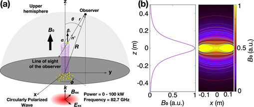
Figure 1. (a) Coordinate system of the calculation where multi-electron (Ne = 100) with cyclotron motion in static magnetic mirror field is accelerated by the RHCP wave. The z component of the magnetic mirror field is the positive direction. The angle α between the line of sight of the observer and the propagation direction of the electron is also defined. (b) Statically applied magnetic mirror field structure used by the calculation with a normalized magnetic field strength by the maximum value on the optical axis at the origin, which is 2.286 T. Left is the spatial distribution on the optical axis. Right is the spatial distribution on xz-plane.
Download figure:
Standard image High-resolution imageIn this calculation, the ordinary differential equation in equation (23) is numerically solved by fourth-order Runge–Kutta method for each electron to obtain the electron trajectory. After that, the calculated trajectory information is substituted into the Liénard–Wiechert potential as shown below to calculate the radiation field created by each electron as well [29, 30]

with

where E ( R , t) is an electric field on the observer point, ɛ0 is dielectric constant of the vacuum, r is the vector toward the observer from electron position, and n ' is the unit vector toward observer from the position of the electron. t' is retarded time. Here, the retarded time and the observer time are explicitly distinguished in equation (27). Note that the retarded time t' is the time frame of electron motion and this is calculated at first on the t' time frame. And then, the advanced time t is calculated by equation (28) as observer time frame. The radiation field is observed on the upper hemisphere where the distance from the origin is | R | = 3 m.
3.1. Electron trajectory in the electromagnetic wave
To clarify the effect of the external electromagnetic field, we calculate the two cases where the external electromagnetic field is applied or is not applied to the electron.
Figures 2(a)–(g) show the trajectory information and some parameters of single electron when the external RHCP wave is not applied, that is Pex = 0 kW. It can be seen as shown in figures 2(a) and (b) purple line that the electron travels along the magnetic mirror field, and the Larmor radius decreases as the magnetic field increases (figure 2(e) is for the magnetic field strength). Also, the Larmor radius increases as the magnetic field decreases. In addition, ωce and ωce,γ increase/decrease as the magnetic field decreases/increases. However, there is no significant difference between ωce and ωce,γ . Note again that the ωce,γ is represented by the relativistic electron cyclotron frequency along the electron trajectory with the magnetic field as shown in figure 2(e). Obviously, the kinetic energy as shown in figure 2(g) does not change because there is no energy transfer from the external electromagnetic field. Here, the kinetic energy was calculated by the definition below:

Furthermore, although the change of the velocity/acceleration in the z direction is quite small, it changes corresponding to the change of the velocity/acceleration in xy-direction so as to preserve the magnetic moment. As there is no external electromagnetic field, electrons simply have pure cyclotron motion. Regarding figure 2(h), we will discuss this below.
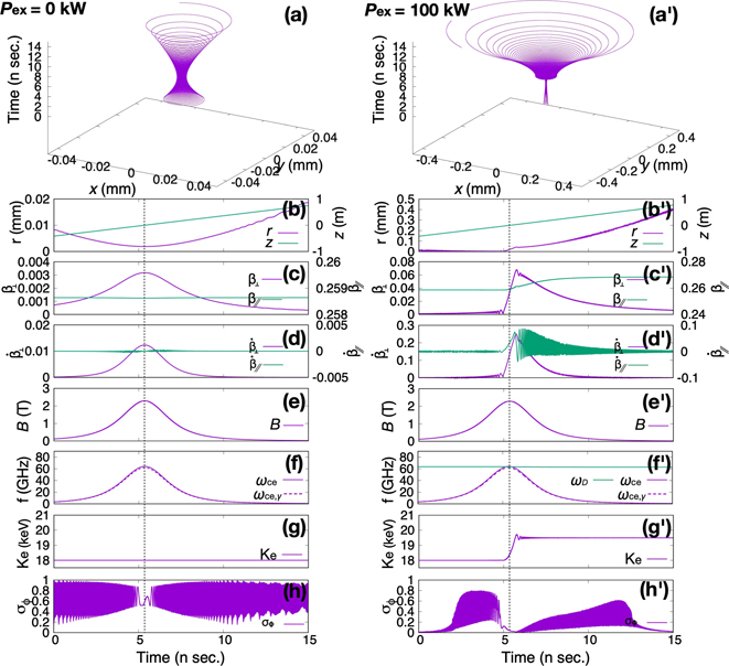
Figure 2. Trajectory information and some parameters when the electron's energy in z-direction has 18 keV. Without prime is Pex is 0 kW and with prime is Pex is 100 kW. (a) and (a') Electron trajectory. (b)–(d) and (b')–(d') Trajectory information concerning positions, velocities, and accelerations. (e) and (e') The magnetic field strength along the electron trajectory. (f) and (f') Electron cyclotron frequency along the electron trajectory. ωD means the Doppler-shifted frequency of the RHCP wave seen from the electron. When ωce = ωD is satisfied, the resonance occurs. (g) and (g') Kinetic energy of the electron. (h) and (h') Standard deviation representing the angle variation between the perpendicular velocity vector and the electric field vector.
Download figure:
Standard image High-resolution imageFigures 2(a')–(g') show the trajectory information and some parameters of single electron when the power of the external RHCP with Pex = 100 kW is applied. As shown in figures 2(a') and (b') purple line, the electron travels along the magnetic mirror field, and the Larmor radius decreases as the magnetic field increases (figure 2(e') is for the magnetic field strength). However, it can be seen that the Larmor radius suddenly increases just after 5 n sec. This is because the electron passes through the resonance magnetic field as shown in figure 2(f'). Since the electron is moving with relativistic velocity in the z direction, the electron sees the RHCP wave with Doppler-shifted frequency ωD (defined below), which is lower than the original frequency of the RHCP wave.

Thus, the resonance occurs when the relationship where ωce = ωD is satisfied. This is because the parallel component of the γ:  , the dispersion relation in vacuum: kc/ω = 1, and the resonance condition: ω = ωce,γ
+ kv∥ directly leads to the relation below [31]:
, the dispersion relation in vacuum: kc/ω = 1, and the resonance condition: ω = ωce,γ
+ kv∥ directly leads to the relation below [31]:

As shown in figure 2(g'), the kinetic energy of the electron spikes when the electron passes through the resonance field. Meanwhile, the velocities and the accelerations in perpendicular direction and parallel direction also have spikes as shown in figures 2(c') and (d'). After passing through the resonant field, in the velocities it can be seen that the perpendicular velocity is gradually decreasing in time, while the parallel velocity is gradually increasing with time. This is because the magnetic moment must be conserved in the magnetic mirror field. Following these phenomena, the accelerations increase/decrease in time. Note that the acceleration in z-direction appears in average, but it is not monotonically. However, in the case of larger velocity in z-direction, the duration time for interaction where the Doppler-shifted frequency of the RHCP wave seen from the reference frame of the electron and the electron cyclotron frequency coincide with each other is very short, thus the resonance time is also short. That is, the energy gain is not large.
The above explanation was the motion per single electron, but this mechanism applies in the same way to other electrons. As mentioned, the phase of the ECE from the multi-electron system is usually incoherent due to the random rotation phase of each electron. However, when the external field is applied and resonance occurs, coherent radiation can be obtained. This is because the electrons are spatially coherent with experimentally applied electromagnetic wave. Here, we define the quantities below:


where  of equation (32) is the cosine component of the angle between the perpendicular velocity vector of each electron and the externally applied electric field vector. And, the over-line of the cosine in (33) represents the average of equation (32) for each electron. That is, σϕ
means the standard deviation. Figure 3(a) shows the spatially incoherent state. That is,
of equation (32) is the cosine component of the angle between the perpendicular velocity vector of each electron and the externally applied electric field vector. And, the over-line of the cosine in (33) represents the average of equation (32) for each electron. That is, σϕ
means the standard deviation. Figure 3(a) shows the spatially incoherent state. That is,  is randomness by each electron in an arbitrary z plane at the time of t = t0 before resonance. However, in the state where the resonance occurs at t = t1 as shown in figure 3(b),
  has the same value for all electrons in any z plane. Note that the direction of the perpendicular velocity vector and the electric field vector in each z plane are different. In this way, when the coherent electron state in space and gyro-phase is produced, the radiation fields from each electron are superposed with the same phase, and coherent radiation can be obtained. This is because the superposed radiation field also propagates at the same speed as the externally applied electric field. As shown in figure 2(h), it can be seen that the standard deviation is not zero at any time, that is, the angle between the perpendicular velocity vector and the electric field vector are completely different. Note that although the electromagnetic wave is not applied in figure 2(h), dummy
E
ex with 0 kW, which is not affected by electrons, is used for the calculation of σϕ
. Also, as shown in figure 2(h'), the standard deviation becomes almost zero at the resonance. That is, the angle between the perpendicular velocity vector and the electric field vector are the same at any z plane, but the values are different at other times. From this, it was confirmed that by applying the external field into a multi-electron system, electrons motion can be controlled and the spatially coherent electrons state can be produced as well.
has the same value for all electrons in any z plane. Note that the direction of the perpendicular velocity vector and the electric field vector in each z plane are different. In this way, when the coherent electron state in space and gyro-phase is produced, the radiation fields from each electron are superposed with the same phase, and coherent radiation can be obtained. This is because the superposed radiation field also propagates at the same speed as the externally applied electric field. As shown in figure 2(h), it can be seen that the standard deviation is not zero at any time, that is, the angle between the perpendicular velocity vector and the electric field vector are completely different. Note that although the electromagnetic wave is not applied in figure 2(h), dummy
E
ex with 0 kW, which is not affected by electrons, is used for the calculation of σϕ
. Also, as shown in figure 2(h'), the standard deviation becomes almost zero at the resonance. That is, the angle between the perpendicular velocity vector and the electric field vector are the same at any z plane, but the values are different at other times. From this, it was confirmed that by applying the external field into a multi-electron system, electrons motion can be controlled and the spatially coherent electrons state can be produced as well.
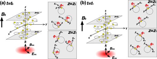
Figure 3. Relationship of the angle between the perpendicular velocity vector of each electron and the externally applied electric field vector. (a) Incoherent spatial distribution of electrons. (b) Coherent spatial distribution of electrons.
Download figure:
Standard image High-resolution image3.2. Observation of the ECE with helical wavefront
We obtained the trajectory information of electrons with cyclotron motion in the magnetic mirror field with and without external RHCP wave. The radiation field can be calculated by using this trajectory information. In this calculation, the radiation is calculated at the distance from the origin | R | = 3 m. By substituting the trajectory information into Liénard–Wiechert potential in equation (27), we can calculate the radiation field. In this calculation, we focus on the radiation observed at the paraxial region such as θ = 0, 10, and 20 deg. because coherence of the radiation depends on the observer position from the optical axis. When the observer is located in the paraxial area, coherency can be maintained. However, the coherency cannot be maintained when the observer position is outside the paraxial area. This is due to the change of the distance between observer and electron caused by random electron distribution in xy plane. That is, electrons distribution does not affect the distance between each electron and the observer, even though they are distributed randomly on xy plane in the case where observer is located in paraxial area. In the case where the observer is located outside the paraxial area, we will be able to discuss this somewhere else.
Figure 4 shows the time variation of the spectrum observed at each θ on ϕ = 0. Taking the retarded time into account, the radiation arrives to the observer in approximately 10 n sec. In this calculation, white noise is added as the background noise. There are two reasons why we calculated that with adding the noise. One is that ECE measurements are often performed in such a detection or system noise environment. The other is to clearly describe and illustrate the essential physical phenomena. The meaning of the latter is that in order to improve the frequency resolution in figure 4, we performed the zero padding before performing fast Fourier transform (FFT). However, when FFT is performed, the artificial periodic spectra appear due to the discontinuity between the actual signal and the zero signal. In order to suppress the effect of the discontinuity, we have multiplied window function. However, the discontinuity could not be eliminated completely even though we selected better window function. Nevertheless, since the intensity of the spectrum caused by the discontinuity is small, it is possible to make a distinction from the actual physical phenomena and the artificial spectra by adding the white noise. The added intensity of the white noise is selected in order to exceed the higher harmonics spectra before resonance.
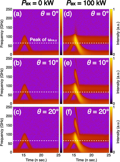
Figure 4. Time variation of the spectrum observed on the upper hemisphere at the distance from the origin | R | = 3 m, each θ on ϕ = 0. The spectra intensity are measured by log scale.
Download figure:
Standard image High-resolution imageFigures 4(a) to (c) show the case where Pex is not applied. As can be seen, the fundamental radiation is only observed at each θ. However, this does not mean that higher harmonics are not generated. The level of the higher harmonics are under the white noise because the noise level is selected in order to exceed the intensity of higher harmonics as we mentioned above. What we would like to emphasize in this paper is that when a resonant external electromagnetic field is applied, the gyro-phase of electrons are controlled, and coherent ECE is expected to be observed as shown below. In addition, the time change of the frequency is observed, which is basically due to the change of the cyclotron frequency, but the observed frequency is actually higher than the cyclotron frequency. This is due to the Doppler effect. Details will be described later.
Figures 4(d) to (f) show the case where Pex = 100 kW is applied. In the common points in every θ, the spectrum with center of 82.7 GHz appears. This is because the electron has trochoidal motion by the effect of externally applied RHCP wave in the weaker magnetic field. That is, although the electron has the cyclotron motion overall, the cyclotron motion is locally controlled by the RHCP wave because the acceleration direction of the electron is mainly decided by the first term on equation (23) in the weaker magnetic field. Also, just after passing through the resonance field (approximately 15 n sec.), radiation intensity is extremely increased. In particular, in the higher harmonics radiation, the radiation is observed above the noise level. This is because electrons motions become spatially coherent due to resonance, and coherent radiation is obtained.
In addition, as can be seen, the fundamental radiation only appears at θ = 0, while higher harmonics appear at other θ. Since θ = 0 corresponds to the optical axis, this suggests that higher harmonics do not have intensity on the optical axis, which is one of the characteristics of the radiation with a helical wavefront.
Here, we will explain the time variation of the observed frequency depending on θ. As mentioned briefly, the time variation of the observed frequency mostly depends on the cyclotron frequency. However, higher frequency compared with the original cyclotron frequency is observed. This can be explained by transverse Doppler effect as follows [29]:

where α is the angle between the line of sight of the observer and the propagation direction as shown in figure 1(a). Figure 5 shows the time variation for the Doppler-shifted frequency calculated by equation (34) observed on the upper hemisphere when the magnetic field is set to 2.286 T and the electron has velocity in z-direction which corresponds to 18 keV. In this case, the electron has the relativistic velocity in z-direction, and the observer located on the upper hemisphere receives the Doppler-shifted radiation frequency. As can be seen when θ is small, the observer receives radiation with blue-shifted frequency larger than ωce,γ . In this calculation of the Doppler effect, the electron motion is only considered to be the z-direction, that is, the cyclotron motion in xy-direction is neglected. Then, the spectra have no Doppler broadening. However, the calculation of the radiation from the electrons in figure 4 are included in all of the electron's motion, which appear to have fluctuation for the observer. Therefore, the spectra have Doppler broadening. Note that the observed frequency will be gradually decreasing compared with θ = 0 by becoming θ larger.
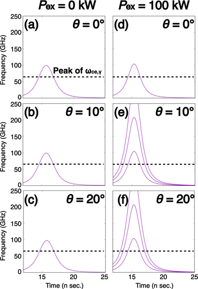
Figure 5. Time variation of the Doppler-shifted frequency calculated by equation (34) observed at each θ. In this calculation, the electron motion is only considered the z-direction.
Download figure:
Standard image High-resolution imageFinally, we will explain the phase structure of the calculated ECE spectra. We obtained the result that the intensity of higher harmonics does not exist on the optical axis. In order to demonstrate that this radiation has helical wavefront as well as the donut-shaped intensity distribution, we calculate the phase difference of the measured radiation at two spacial points by using the definition below

In this study, we focus on the phase difference between ϕ = 0 deg. and ϕ = 90/180 deg., that is, fph(ϕ = 90/180) is represented on figures 6 and 7.
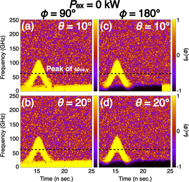
Figure 6. Time variation of the phase difference between ϕ = 0 and ϕ = 90/180 deg. observed on the upper hemisphere at the distance from the origin | R | = 3 m, each θ when Pex is 0 kW. The phase differences are not to be shown in the case where θ = 0 because the phase differences are meaningless.
Download figure:
Standard image High-resolution image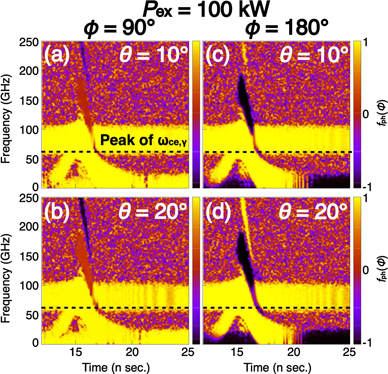
Figure 7. Time variation of the phase difference between ϕ = 0 and ϕ = 90/180 deg. observed on the upper hemisphere at the distance from the origin | R | = 3 m, each θ when Pex is 100 kW. The phase differences are not to be shown in the case where θ = 0 because the phase differences are meaningless.
Download figure:
Standard image High-resolution image
Figure 6 shows the phase difference calculated by equation (35) when Pex is 0 kW. Note that the phase differences are not to be shown in the figure in the case where θ = 0 because the phase differences are meaningless. In other θ, as mentioned, when in the case where Pex is 0 kW, only the fundamental radiation is calculated. Therefore, it can be seen that fph(ϕ) is 1 at all θ except for θ = 0 deg. That is, the phase difference is zero in fundamental radiation.
Figure 7 shows the phase difference calculated by equation (35) when Pex is 100 kW. Note that the phase differences are not to be shown in the figure in the case where θ = 0 because the phase differences are meaningless as well. In other θ, it can be seen that fph(ϕ) also changes along the spectrum of fundamental and harmonics radiation. In the case of fundamental radiation, it can be seen in both figures that fph(ϕ) is 1 at all θ. That is, the phase difference is zero in fundamental radiation. This indicates that the fundamental radiation is just a wave with a spherical equiphase front. In the case of second harmonic radiation, it can be seen that when ϕ = 90 deg., fph(ϕ) is 0 at all θ except for θ = 0 deg., which indicates that the phase difference is 90 deg., while when ϕ = 180 deg., fph(ϕ) is −1 at all θ except for θ = 0 deg., which indicates that the phase difference is 180 deg. That is, the phase in second harmonic radiation changes 360 deg. around the optical axis. In addition, in the case of third harmonic radiation, when ϕ = 90 deg., fph(ϕ) of the third harmonic is −1, which indicates that there is a phase difference of 180 deg., while when ϕ = 180 deg., fph(ϕ) is 1 again at all θ except for θ = 0 deg., which indicates that the phase difference is 360 deg. That is, the phase in third harmonic radiation changes by 720 deg. around the optical axis. In this way, it was shown that the harmonics radiation has the phase difference with 90(n − 1) between ϕ = 0 deg. and ϕ = 90 deg. or with 180(n − 1) between ϕ = 0 deg. and ϕ = 180 deg. These results suggest that ECE has a helical wavefront from the characteristics of donut-shaped intensity distribution and azimuth-dependent phase structure.
4. Summary
In this study, we carried out a numerical calculation regarding cyclotron emission from multi-electron system in static magnetic mirror field accelerated by externally applied circularly polarized wave. In this calculation, we showed that when electrons were in resonance state, a coherent electron distribution in space and gyro-phase could be produced. As a result, a coherent ECE with intensity above noise level was calculated. This was because of the superposed the electric field created by each electron. In addition, only spectrum of the fundamental radiation appeared at θ = 0 although the higher harmonics was observed at any other θ. Since θ = 0 corresponds to the optical axis, this showed that higher harmonics do not have intensity on the optical axis. Also, in the phase difference between two spatial points, we showed that the phase difference has 90(n − 1) or 180(n − 1) at between ϕ = 0 deg. and ϕ = 90/180 deg in all θ except for optical axis. These results showed that only higher harmonics radiation have the helical wavefront with donut-shaped intensity distribution. In this calculation, there is no collision between electrons because we only considered each electron's motion in vacuum independently. Actually, in the case where the power of the externally applied electromagnetic wave is considered to be sufficiently larger than the interaction force between electrons under the realistic electron density considered, collisions might not have to be considered as well. Nevertheless, we are also attempting to calculate by particle-in-cell simulation for more precise calculations.
Data availability statement
All data that support the findings of this study are included within the article (and any supplementary files).