


Abstract
The practical security of a continuous-variable quantum key distribution (CVQKD) system is compromised by various attack strategies. The existing countermeasures against these attacks are to exploit different real-time monitoring modules to prevent different types of attacks, which significantly depend on the accuracy of the estimated excess noise and lack a universal defense method. In this paper, we propose a defense strategy for CVQKD systems to address these disadvantages and resist most of the known attack types. We investigate several features of the pulses that would be affected by different types of attacks, derive a feature vector based on these features as the input of an artificial neural network (ANN) model, and show the training and testing process of the ANN model for attack detection and classification. Simulation results show that the proposed scheme can effectively detect most of the known attacks at the cost of reducing a small part of secret keys and transmission distance. It establishes a universal attack detection model by simply monitoring several features of the pulses without knowing the exact type of attack in advance.
Export citation and abstract BibTeX RIS

Original content from this work may be used under the terms of the Creative Commons Attribution 4.0 licence. Any further distribution of this work must maintain attribution to the author(s) and the title of the work, journal citation and DOI.
1. Introduction
Quantum key distribution (QKD) [1] is one of the most important application of quantum technologies, which enables two distant parties, Alice and Bob, to exchange secret keys in an untrusted environment without being eavesdropped by an eavesdropper, Eve its theoretical unconditional security is guaranteed by the fundamental laws of quantum mechanics [2, 3], which based on some assumptions that Alice and Bob's device are supposed to behave according to a perfect model. However, there are some deviations between the theoretical perfect assumptions and practical QKD implementations, such deviations may bring loopholes and enable Eve to break the security by stealing information from the legitimate parties [4–6].
According to different implementation methods, QKD can be divided into two types: discrete-variable (DV) QKD [7, 8] and continuous-variable (CV) QKD [9–11]. Compared with DVQKD, CVQKD has higher secret key rate and better compatibility with the current optical networks [12]. Gaussian modulated coherent state (GMCS) protocol is the most popular CVQKD scheme [13, 14], which has been proven theoretically secure against collective attacks [15–17]. However, the security of the practical GMCS CVQKD can be broken by some practical attack strategies, such as Trojan-horse attacks [18, 19], wavelength attacks [20, 21], calibration attacks [22], local oscillator (LO) intensity attacks [23], saturation attacks [24], and homodyne-detector-blinding attacks [25]. The main idea of these attacks is to exploit the imperfections of optical devices to bias the excess noise estimation, and the essence of the corresponding countermeasures is to add suitable real-time monitoring modules on the system, which significantly depend on the accuracy of the estimated excess noise and the calculated precision of a low bound of optical features disturbance for Eve successfully concealing herself [26]. However, in practice there are some natural fluctuations in the legitimate light as well as real detectors and electronics, Alice and Bob have to implement multiple iterative calculations to obtain an accurate estimation. In addition, the estimation procedure is usually implemented after the key transmission process is completed, once an attack is found the whole key data should be discarded, wasting a lot of time and resources. Moreover, in actual systems we do not know in advance which kind of attack Eve will launch, so we need a universal defense solution which can resist as many attack types as possible.
In this paper, we propose a defense strategy for CVQKD systems to address the disadvantages mentioned above. We investigate several typical features of the pulses that would be effected by the attacks, and the deviations of these features between normal unattacked pulses and abnormal attacked pulses. A set of feature vectors labeled by different attack types is constructed to train an artificial neural network (ANN). The trained ANN model can automatically detect abnormal feature vectors and classify them into different attack types. Consequently, a universal attack detection model is established, which can recognize most of the known attack types by using only one forward propagation calculating process. The secret keys received by Bob can be sequentially input into the model, and the transmission process will be aborted immediately once abnormal data is found. In this way Bob does not need to wait until the key transmission process is complete to check if the system is attacked. In our work, we mainly consider three typical attack strategies against GMCS CVQKD systems with homodyne detection, including the calibration attack, the LO intensity attack, and the saturation attack. In addition, two types of hybrid attack strategies [25, 27] is also investigated. Individual wavelength attacks [20, 21] are not considered here because they are only effective for heterodyne detection CVQKD systems. For one-way GMCS CVQKD systems, isolators and wavelength filters are the most suitable countermeasures against Trojan-horse attacks, thus the Trojan-horse attack is also not contained in our work.
2. Learning for automatic attack classification
2.1. Feature extraction of optical pulses
In a GMCS CVQKD protocol, Alice prepares a train of coherent states |XA + iPA⟩ where the quadrature values XA and PA subject to a bivariate Gaussian distribution with variance VAN0. Here N0 represents the shot noise variance which corresponds to the variance of the homodyne detector output when the input signals are vacuum states. Then Alice sends the prepared states to Bob with a strong LO of intensity ILO by using polarization multiplexing technique. The receiver Bob measures one of the quadratures of the signal states by performing a homodyne detection, with the help of the LO as a phase reference. After this process, Alice and Bob obtain two strings of correlated data x = {x1, x2, ..., xN} and y = {y1, y2, ..., yN}, where x represents the quadrature value modulated by Alice (XA or PA) and y represents the quadrature value measured by Bob (XB or PB). We note that


where T and η are the quantum channel transmittance and the efficiency of the homodyne detector, respectively. Vel = velN0 is the detector's electronic noise and ξ = ɛN0 is the technical excess noise of the system. In a practical CVQKD system, there are several features could be affected by different attack strategies, such as the intensity ILO of the LO, the shot noise variance N0, the mean value  and variance Vy of Bob's measurement. Table 1 shows the impacts of different attack strategies on the measurable features. We find that the first four types of attacks affect different features. Although the last attack strategy and the saturation attack act on the same features, they have different degree of impact (more details can be found in the appendix
Table 1. Impacts of different attack strategies on measurable features. The symbol '√' under the features indicates that the corresponding feature will be changed by the corresponding attack.
| Features | | Vy | ILO | N0 |
|---|---|---|---|---|
| LO intensity attack [23] | — | √ | √ | √ |
| Calibration attack [22] | — | √ | — | √ |
| Saturation attack [24] | √ | √ | — | — |
| Hybrid attack 1 [27] | — | √ | √ | — |
| Hybrid attack 2 [25] | √ | √ | — | — |
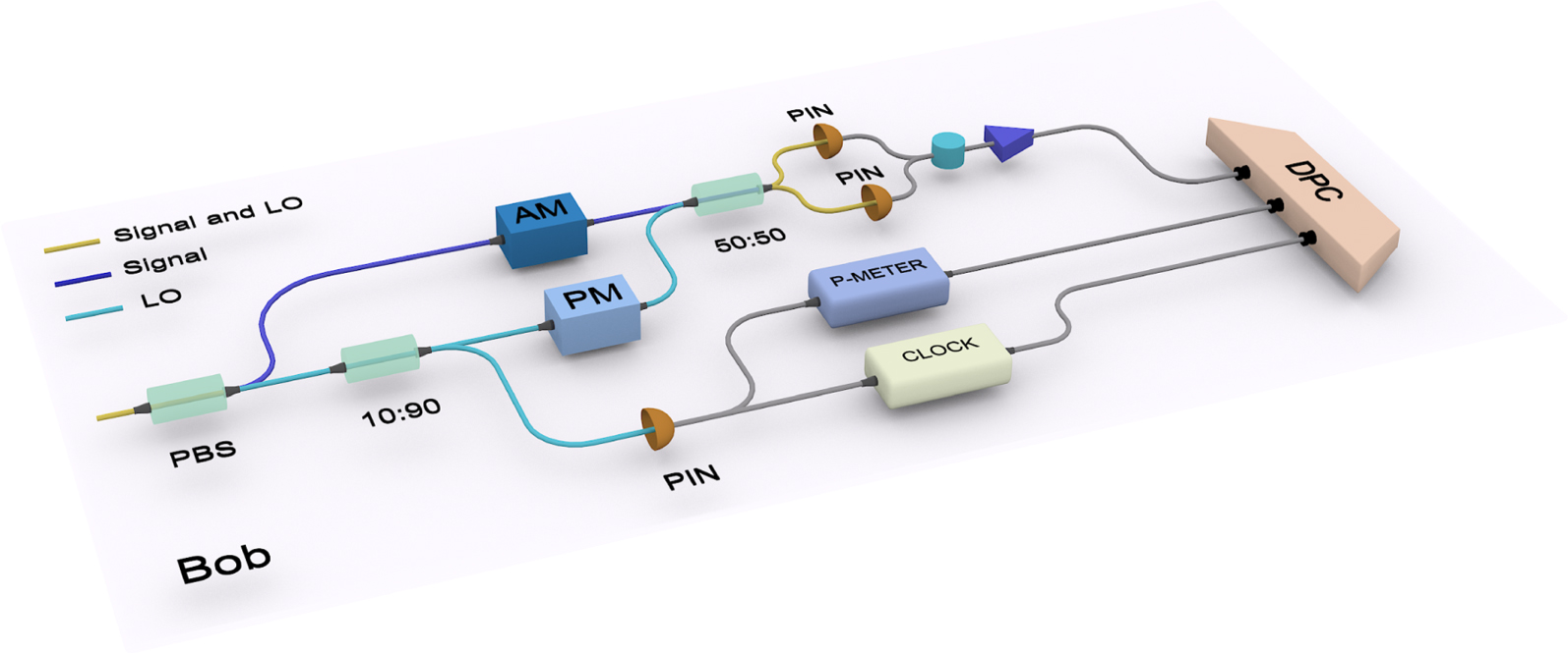
Figure 1 shows the schematic diagram of Bob's detection setup that is used for simultaneously measuring the features mentioned above. Firstly, the signal and LO pulses are demultiplexed by using a PBS. Then, an AM is applied on the signal path to randomly set a maximum attenuation with a probability of 10% for real-time shot-noise estimation, and the remaining signal pulses are not attenuated. Meanwhile, the LO pulses are split by a 90:10 beam splitter, part of which are used for homodyne detection and part of which are used for power monitoring and clock generation. After that, the analog measurement results are fed in the DPC for sampling and attack detection. We assume that Bob receives N pulses in a communication process and all these pulses can be divided into M blocks. For each block, we can calculate the mean and variance, the LO average power, and the shot noise variance. By this way, a feature vector  is constructed to represent the corresponding block. M feature vectors
  of the M blocks form the input of the ANN model, as shown in figure 2. The values of the feature vector are various under different types of attacks, since different attacks act on different features and change the values of them in different ways. According to the approximation theorem of the neural networks, it is possible to infinitely approximate to any given bounded continuous function on a given domain with a neural network [28]. It suggests that the neural network can fully learning the behaviours of the attacks based on the established feature vectors. It is worth noting that although there may be errors between the feature values of each block and these values of the whole data, the neural network can still use them to distinguish attacks because the errors under different attacks is also different.

Figure 1. Schematic diagram of Bob's detection setup for protecting a CVQKD system against attacks. PBS: polarization beam splitter. AM: amplitude modulator. PM: phase modulator. PIN: PIN photodiode. P-METER: power meter. CLOCK: clock circuit used to generate clock signal for measurement. DPC: data processing center used to sample analog signal, attack detection and raw key distillation.
Download figure:
Standard image High-resolution image
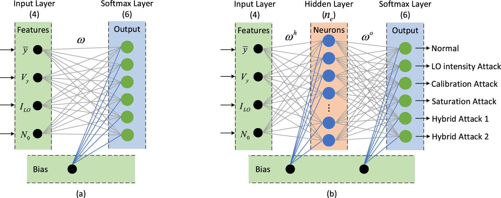
Figure 2. ANN-based quantum attack detection model. The circles represent the artificial neutrons in each layer and the lines represent the weights of the neutrons output to the next layer. (a) A linear ANN model without the hidden layer which can only solve linear separable problems. (b) A nonlinear ANN model with a hidden layer to classify different types of quantum attacks.
Download figure:
Standard image High-resolution image2.2. Artificial neural network establishment for attack classification
In this section, we introduce how to establish the ANN attack detection model based on feature vectors. ANN is a popular machine learning technique inspired by the biological neural network in the human brain [29]. As shown in figure 2, an ANN consists of several layers and each layer contains many neurons, ANN sends the weight values of each neuron as output to the next layer after processing with inputs from neurons in the previous layer. Our target is to derive an output vector  according to the input vector
  by constructing a classifier, which is represented by a function
  . The construction of the classifier is based on multiple training iterations on a training set
  . In our scheme, the input vector
  consists of the features listed in table 1, the output vector
  consists of a set of probability values, which represent the probability that the current input data belongs to each attack type. Figure 2(a) is a linear ANN model without hidden layers which can only solve linear separable problems. In order to applicable to distinguish different types of attacks, we join a hidden layer between the input layer and the output layer, and further construct a nonlinear ANN multi-classifier by using a softmax function. The number of neurons in the hidden layer can be adjusted for optimal performance. Figure 2(b) shows the nonlinear ANN multi-classifier that contains three layers: input layer, hidden layer and softmax layer (output layer). Each neuron in the current layer is a linear combination of neurons in the previous layer with weight ω and bias b. For example, the relationship between the input layer and the hidden layer is expressed as

where  is the jth output of the hidden layer, ui is the ith element of the input vector
  ,
,  is the jth bias unit input into the hidden layer,
  is the weight between the ith element of the input layer and the jth element of the hidden layer which will be iterative optimized in the training process. σtanH is the activation function which is defined as [30, 31]

In a similar manner the relationship between the hidden layer and the output layer is obtained by

where σS is the softmax function which is given by

 is the weight between the ith element of the hidden layer and the jth element of the output layer,
  is the jth bias unit input into the output layer,
  is the jth element of the output layer, and the sum of the output
  . The final output
  of the ANN model consists of six probability values, which represent the probability that the vector
  belongs to each class. In the training process, the back-propagation algorithm is used to quickly solve the partial derivatives of the objective function on the internal weights in the network [32], and the weights is accordingly adjusted by using the stochastic gradient descent optimization algorithm [33]. Finally, an ANN model that matches the target output is learned by minimizing the objective function
  when the target class is j.
2.3. Training and testing process
According to the data preparation process described in the appendix


where TP (true positive) denotes the number of the feature vectors that belong to an certain attack type are identified as such attack, FP (false positive) denotes the number of the feature vectors that do not belong to an certain attack type are identified as such attack. FN (false negative) denotes the number of the feature vectors that belong to an certain attack type but are not identified as such attack. TN (true negative) denotes the number of the feature vectors that do not belong to an certain attack type and are not identified as such attack. In general, a fine ANN classifier can achieve high values of precision and recall, and low values of FPR and FNR. In the testing stage, 'one vs others' method is employed to evaluate the performance of the classifier. For example, when calculating the precision of detecting LO intensity attack, the LO intensity attack-related feature vectors are considered as positive instances, while the other five types of vectors are considered as negative instances, which simplifies the multi-class problem to a binary-class problem.

Figure 3. Training and testing procedure of the ANN model.
Download figure:
Standard image High-resolution image3. Performance analysis
3.1. Implementation details
We implement ANN training and testing on Matlab R2019b, with the help of neural network toolbox. The memory and processor of our computer are 16 GB and Intel Core 4.0 GHz CPU, respectively, and the operating system is Windows 10 Professional. In the experiments the learning rate and error goal of ANN are set as 0.01, and the maximum iterations is 500. The data set size of each attack type is N = 1 × 10⁷ and the number of pulses in each block is Q = 1 × 10⁴, therefore, the data set of each attack type can be divided into M = 1000 feature vectors, 6 types of data constitute 6000 feature vectors. It is worth noting that too small M value will make the ANN model unable to learn the characteristics of each attack type well, and too large M value will bring a large statistical error to the feature values of each block. In practical implementation, the value of M can be optimized by using the grid search algorithm, which is the most widely used strategies for hyper-parameter optimization [34]
3.2. Performance of attack classification for CVQKD system
In this section we analyze the performance of the ANN model for attack detection and classification. Firstly, we introduce principal component analysis [35] to map the collected 6000 feature vectors of six types of data into a 2D metric space, as shown in figure 4(a). We can find that the feature vectors of the calibration attack, the saturation attack and the hybrid attack 2 are very different from the normal unattacked vectors, whereas the feature vectors of the LO intensity attack and the hybrid attack 1 are close to the normal vectors and hard to be separated by statistical analysis. Figure 4(b) shows the mapped instances after ANN classification, we can see that different types of data are significantly separated by the ANN model. In order to determine the optimal number of neurons ne in the hidden layer, we calculate the values of precision, recall, FPR and FNR of the ANN model for attack classification, all of the results are the average of 20 iterations for fear of overfitting and underfitting. As illustrated in figure 5, the precision and recall of the calibration attack, the saturation attack, the hybrid attack 1 and the hybrid attack 2 reach the maximum 1 when the value of ne = 15. For the LO intensity attack under the same condition, the performance of the ANN is the worst with precision and recall of 0.9969 and 0.9961, respectively. This is because the feature vectors of the LO intensity attack is closest to the normal data compared to other attacks. Similarly, the FPR and FNR of the calibration attack, the saturation attack, the hybrid attack 1 and the hybrid attack 2 achieve the minimum value of 0 at ne = 15, but these two values of the LO intensity attack are 6.2 × 10⁻⁴ and 3.9 × 10⁻³, respectively. The performance of ANN classification is relatively stable when the value of ne between 5 and 20, while the precision and recall are low when ne = 1 because the ANN model does not have enough learning ability when the number of neurons in hidden layer is small. In addition, the results of precision, recall, FPR and FNR fluctuate apparently in the condition of ne > 20, because too many neurons in hidden layer greatly increase the complexity of the ANN, thereby neurons in the hidden layer will lose their sensitivity to input signals, and the propagation of information is blocked severely, under this situation the network is easily trapped into a local minimum point and fail to converged to a global minimum within a reasonable number of iterations [36].

Figure 4. (a) The distribution of 6000 feature vector instances consist of 6 types of attack data before ANN classification. (b) The distribution of 6000 feature vector instances consist of 6 types of attack data after ANN classification.
Download figure:
Standard image High-resolution image
Figure 5. (a) Precision of the ANN model for attack classification versus different values of ne. (b) Recall of the ANN model for attack classification versus different values of ne. (c) FPR of the ANN model for attack classification versus different values of ne. (d) FNR of the ANN model for attack classification versus different values of ne.
Download figure:
Standard image High-resolution image3.3. Secret key rate of ANN-based attack defense strategy
In this section, we compare the secret key rates for a CVQKD system that employs the ANN-based attack detection model and for a system that does not employ any countermeasures against attacks. The most commonly used method is the asymptotic secret key rate which is given by [13]

where β is the reverse reconciliation efficiency, IAB is the Shannon mutual information between Alice and Bob, and χBE is the Holevo quantity for Eve's maximum accessible information. The detailed calculation about IAB and χBE can be found in appendix

Figure 6. (a) Secret key rate against collective attacks in the asymptotic and finite-size regime. The solid lines correspond to the secret key rates of the system without any countermeasures, and the dashed lines correspond to the secret key rates of the system employ the ANN-based attack detection model. From left to right, the curves correspond, respectively, to the number of exchanged signals N = 108, N = 1010, N = 1012, N = 1014, and the asymptotic case. (b) Composable secret key rates of a CVQKD system with and without using the ANN-based attack detection model. The solid lines from left to right correspond to the composable secret key rates with and without ANN-based attack detection at transmission distances of 10 km, 20 km, and 30 km, respectively. The dashed lines with the same color as the solid lines are their corresponding asymptotic secret key rates under the same conditions. In all the simulations, the insertion loss of the AM on Bob's signal path is set to a typical value of 2.7 dB.
Download figure:
Standard image High-resolution image4. Conclusion
In this work, we introduced and experimentally addressed a quantum attack defense strategy for CVQKD systems by using ANN. We considered the impacts of existing attack strategies on the measurable features of signal and LO pulses, and established a set of feature vectors label by different attack types as input of an ANN model. According to the realistic assumption of the attacks, the training and testing data is prepared for performance evaluation. Simulation results show that the trained ANN can automatically identify and classify attacks with precision and recall values above 99%. Interestingly, we find that the performance of the ANN model is sensitive to the number of neurons ne in the hidden layer, therefore how to select an appropriate values of ne is important in practical implementation. Comparing with a system that does not adopt any anti-attack countermeasures, our scheme slightly diminished the secret key rate and transmission distance, but it constructed an overall defense model to anti most of the known attack strategies, significantly improves the security of the system.
Acknowledgments
This work was supported by the National Natural Science Foundation of China (NSFC) (61972418, 61977062, 61872390, 61871407 and 61801522) and the National Natural Science Foundation of Hunan Province, China (2019JJ40352).
Appendix A.: Data preparation and realistic assumption of attacks
In order to investigate the performance of the ANN model for attack classification, we need to establish several valid data sets based on a realistic assumption of Alice and Bob's implementation setup, as well as Eve's capability. Firstly, we assume the fixed parameters mentioned above as: VA = 10, η = 0.6, ξ = 0.1N0, Vel = 0.01N0, T = 10−αL/10, where L is the transmission distance which is set as a typical value of 30 km and α = 0.2 dB km−1 is the loss coefficient of the optical fiber. The attenuation values set by Bob are r1 = 1 (no attenuation) and r2 = 0.001 (maximum attenuation). All of these values are selected according to the standard realistic assumption for CVQKD implementations [22, 39]. In a normal condition without any attacks, the mean and variance of the measurement results are given by

where Vi = {V1, V2} corresponds to the values of ri, the LO power ILO at Bob side is set as 107 photons per pulse with 1% fluctuation [26, 40]. Accordingly, the shot noise variance N0 under normal condition is set as 0.4 based on the calibrated linear relationship in [22].
Secondly, we briefly recall the principles of the above-mentioned attack strategies, including the LO intensity attack, the calibration attack, the saturation attack, the hybrid attack 1 and the hybrid attack 2.
- (a)In the LO intensity attack, Eve attacks the signal beam with a general Gaussian collective attack [15, 41] and attacks the LO beam by using a non-changing phase intensity attenuator with attenuation coefficient k(0 < k < 1). By this way, Eve can arbitrarily reduce the excess noise ɛ estimated by Alice and Bob to zero and hide her attack. For computational simplicity, we assume the variable attenuation coefficient k of each LO pulse is the same. Therefore, the variance of Bob's measurement results under this attack can be expressed aswhere
 represents the noise introduced by Eve's Gaussian collective attack, N = (1 − kηT)/k(1 − ηT) represents the variance of Eve's EPR states. Similarly, the shot noise is also deviated from the initial level as .
 - (b)In the calibration attack, Eve intercepts a fraction μ of the signal pulses by implementing a partial intercept-resend (PIR) attack and modifies the shape of LO pulses to control the shot noise estimated by legitimate parties. According to the description in [22], the excess noise introduced by calibration attack is expressed aswhere ξPIR = ξ + 2μN0 is the excess noise introduced by Eve's PIR attack, is the shot noise after calibration attack and N0 is the shot noise before attack. In order to make the excess noise estimated by Alice and Bob close to zero, the ratio must satisfywith μ = 1 and a typical value of. (A.5) indicates that the original shot noise N0 is reduced into by a factor of δ = 1/(1 + 2.1ηT). Therefore, the variance of the measurement results under this attack can be expressed as
- (c)In the saturation attack, Eve exploits the finite linearity domain of the homodyne detection response. In order to saturate Bob's detector, She intercepts all the pulses send by Alice and measures them with heterodyne detection, then displaces the quadratures of the resent coherent states with a value Δ. As shown in [24], the mean and variance of Bob under saturation attack are expressed aswherein which α is the boundary of the linear range of the homodyne detector, and the function erf(x) is the error function defined as
- (d)In the hybrid attack 1, we consider the strategy A that consists of two attack parts. The first part is similar with the LO intensity attack, Eve performs intercept-resend attack to obtain the information sent by Alice and prepares new signal and LO pulses with amplitude and , respectively, where XE and PE are the quadrature values measured by Eve, αLO is the amplitude of the original LO and λ is a real number. In the second attack part Eve prepares and resends two extra coherent pulses with wavelengths different from the typical communication wavelength of 1550 nm, so that makes the shot noise measurement results seem normal. The variance of Bob's measurement results is given bywhere D depends on the intensities Is, Ilo and wavelengths λs, λlo of the extra two pulses. The shot noise level and excess noise estimated by legitimate parties are expressed as
- (e)In the hybrid attack 2, Eve performs a full intercept-resend attack, and inserts external pluses into the signal port of Bob's homodyne detector along with the re-prepared signals. The pulse width and repetition rate of the external pulses are the same as the pulses sent by Alice. But the wavelength of them is slightly different with Alice's signals, in order to saturate Bob's homodyne detector output. In this way, the external light causes a non-negligible offset on the measurement results of Bob, which is given bywhere Text is the overall transmission of Bob's homodyne detector regarding the external pulses and is related to the wavelength of the pulse, Iext is the number of photons per pulse of the external light, and Dext is normalized in. The excess noise of the system under this attack becomeswhere ξIR = 2N0 is the noise caused by the intercept-resend attack, and ξext is the noise caused by the external light, which is related to the value of Iext.


Thirdly, we define the values of the parameters employed in different attack types. For the LO intensity attack, we set the LO fluctuation rate 1 − k as 0.05 since the analysis in [23] shows that Eve can obtain the full secret keys with an LO fluctuation rate of 0.05 at a transmission distance of 30 km. For the calibration attack, the value of δ is set according to the specific values of η and T based on the equation δ = 1/(1 + 2.1ηT). For the saturation attack, the value of α is set to  and the value of Δ is set to
  since the analysis in [24] shows that the value of Δ should close to α for better attack effect. For the hybrid attack 1, the values of D and λ are selected according to the equations (A.15) and (A.16) to make
  and
and  arbitrarily cloze to zero. For the hybrid attack 2, the value of Text is set as 0.49, and the value of Iext is selected according to the specific parameter values to make the estimated excess noise smaller than the null key threshold.
Finally, in order to explain the data preparation process more clearly, we summarize the parameters used to generate the data sets for the normal unattacked situation and five attacks strategies, as shown in table 2. The size of each type of data set is 1 × N, where 90% of the values in each data set are generated based on ri = r1, and 10% of the values are generated based on ri = r2. For example, we generate two groups of normal data, the first group is y1 = {y1, y2, ..., yN−0.1N} which follows a Gaussian distribution with zero mean and variance V1 = r1ηT(VAN0 + ξ) + N0 + Vel, the second group is y2 = {y1, y2, ..., y0.1N} which follows a Gaussian distribution with zero mean and variance V2 = r2ηT(VAN0 + ξ) + N0 + Vel. Combining the two groups of data evenly and obtaining ynormal = {y1, y2, ..., yN}, which means that 10% of the data in ynormal is generated for shot noise estimation. In order to establish feature vectors, we divide ynormal into M blocks {b1, b2, ..., bM}. In each block bm, the values from y1 are used for calculating the mean m and variance  of this block, the values from y2 are used for estimating the shot noise variance
  of this block. The LO power of this block is obtained by calculating the average power of the pulses in the current block. Among all of the data sets, yhyb2 is generated a little differently from the others. Firstly, we generate two groups of data y1 and y2. Then, add a value of
  on them, respectively. For each value yi in these two groups, perform the following calculation, as

Finally, combine the resulting two groups of values evenly and obtain yhyb2. It is worth noting that we did not describe how to set the value of shot noise N0 in table 2 because N0 can be calculated based on the specific data in each block.
Table 2. Parameters used to generate the data sets of the normal unattacked data and the five attack strategies.
| Data sets | Parameters for data generation |
|---|---|
| ynormal | , Vi, ILO |
| yLOIA | ,  , kILO , kILO |
| ycalib | ,  , ILO , ILO |
| ysat | sat,  , ILO , ILO |
| yhyb1 | ,  , ILO/λ , ILO/λ |
| yhyb2 | , Vi, ξext, Dext, α, ILO |
Appendix B.: Calculation of asymptotic secret key rate
The asymptotic secret key rate under collective attacks with reverse reconciliation is given by equation (11), where the mutual information IAB between Alice and Bob is derived from Bob's measured values VB = ηT(V + χtol) and the conditional variance VB|A = ηT(1 + χtol) by using Shannon's equation,

where χtol = χline + χhom/T represents the total noise referred to the channel input. χline = T−1 + ɛ − 1 is the channel-added noise referred to the channel input and χhom = [(1 − η) + vel]/η is the detection-added noise referred to Bob's input. χBE denotes the maximum information available to Eve on Bob's key, which is given by

where mB denotes the measurement of Bob, p(mB) denotes the probability density of the measurement,  denotes Eve's state conditional on Bob's measurement, and S denotes the Von Neumann entropy of the quantum state ρ. In the case of Gaussian attack, equation (B.2) can be simplified to

where G(x) = (x + 1)log2(x + 1) − x log2(x). λ1,2 are the symplectic eigenvalues given by

with


λ3,4 are the symplectic eigenvalues given by

with


The last symplectic eigenvalue λ5 = 1. Based on the above equations, we can obtain the secret key rate of the CVQKD system without taking any countermeasures against attacks. When calculating the secret key rate of our scheme, the insertion loss of the AM on Bob's signal path should be taken into consideration, as well as the 10% pulses used for real-time shot-noise measurement.
Appendix C.: Secret key rate in finite-size scenario
The secret key rate of a CVQKD system considering finite-size effects is given by [37]

where N denotes the number of the exchanged signals between Alice and Bob, and n denotes the number of the signals used for key establishment. m = N − n indicates the number of the remaining signals used for parameter estimation.  PE indicates the failure probability of parameter estimation. △(n) is related to the security of the privacy amplification, which is given by

where  is a smoothing parameter, PA is the failure probability of the privacy amplification procedure, and
  is the Hilbert space corresponding to the variable y used in the raw key. We take
  for secret key rate evaluation since the raw key is encoded on bits.
  represents the mutual information between Bob and Eve, which is determined by the covariance matrix ΓAB of the bipartite state shared by Alice and Bob after the quantum channel, that is

where the matrices  and σz = diag(1, −1). Tmin and ɛmax correspond, respectively, to the lower and upper bound of T and ɛ, which are defined as

with


where  follows
  . Substituting Tmin and ɛmax for the parameters T and ɛ used in equation (B.3), we can obtain the secret key rate in finite-size scenario. In the simulations, the above-mentioned error probabilities are set to

Appendix D.: Secret key rate in composable security
In the composable security framework, the secret key rate of a CVQKD protocol against collective attacks is given by [38]

where rob indicates the robustness of the protocol. f is the function computing the Holevo information between Eve and Bob's measurement results for a Gaussian state with covariance matrix parametrized by  ,
,  , and
, and  , that is

where ν1 and ν2 are the symplectic eigenvalues of the covariance matrix ![$\left[\begin{matrix}{cc}\hfill {{\Sigma}}_{a}^{\mathrm{max}}{\mathbb{I}}_{2}\hfill & \hfill {{\Sigma}}_{c}^{\mathrm{min}}{\sigma }_{z}\hfill \\ \hfill {{\Sigma}}_{c}^{\mathrm{min}}{\sigma }_{z}\hfill & \hfill {{\Sigma}}_{b}^{\mathrm{max}}{\mathbb{I}}_{2}\hfill \end{matrix}\right]$](https://content.cld.iop.org/journals/1367-2630/22/8/083073/revision2/njpaba8d4ieqn51.gif) ,
,  . More explicitly,


Then we define


Assuming that the success probability of parameter estimation is at least 0.99, thereby the robustness of the protocol is rob ⩽ 0.01, and the random variables ||X||2, ||Y||2, and ⟨X, Y⟩ satisfy the following restrains


The parameters △AEP and △ent in equation (D.1) can be obtained by


where d is the discretization parameter.  is a possible security parameter. In the simulations, we choose
  , PE = cor = ent = 10−41, and d = 5 for simplicity.