


Abstract
We solve the magnetostriction strains for B20 helimagnets in the skyrmion crystal phase. By taking MnSi as an example, we reproduce its temperature–magnetic field (T–B) phase diagrams within a thermodynamic potential incorporating magnetoelastic interactions. The calculation shows that the normal strain ε33 undergoes a sudden jump through a conical-skyrmion phase transition at any temperature. The corresponding experimental measurements for MnSi agree quantitatively well with the calculation.
Export citation and abstract BibTeX RIS

Original content from this work may be used under the terms of the Creative Commons Attribution 3.0 licence. Any further distribution of this work must maintain attribution to the author(s) and the title of the work, journal citation and DOI.
1. Introduction
Magnetic skyrmion, a topologically protected spin whirl, has attracted great attention for its potential applications in spintronics devices since its experimental discovery in 2009 [1]. Initially found in a small pocket-like region in the temperature–magnetic field phase diagram of bulk MnSi [1], skyrmions are later widely observed in other B20 bulk materials [2–4], thin films [5–9] and nanostructures [10–14] with enhanced stability. As a magnetic texture, skyrmion is not only affected by application of electromagnetic fields such as bias magnetic field, electric current [15], and laser [16], but also sensitive to non-electromagnetic fields such as temperature gradient [17] and mechanical stresses [3, 18]. While the interaction between skyrmions and the electromagnetic fields or the temperature gradient are well-understood both theoretically and experimentally, the effect of mechanical stress on the skyrmion is not well addressed, even though several previous experiments have proven that mechanical stress is an effective method for controlling the formation and stability of skyrmions [3, 18–24] and even their dynamic properties [25]. More specifically, the ultra-low emergent elastic stiffness [26] of the skyrmion crystal (SkX) observed in FeGe thin films [3] and in MnSi [18] makes it convenient to manipulate with mechanical stresses. Concerning the tensor properties of mechanical stresses and strains, sophisticated manipulation of the properties and stability of magnetic skyrmions may be realized by changing the type of mechanical loading, for which a comprehensive understanding of the interaction mechanism between magnetic skyrmions and mechanical loads is highly required.
The interaction between skyrmions and mechanical loads stem from the intrinsic magnetoelastic coupling in chiral magnets, which in turn affects the mechanical properties of the materials. Before the experimental discovery of SkX, the magnetostriction of a prototype helimagnet MnSi has been studied [27]. It is later found that appearance of the SkX phase leads to a jump of the magnetostriction [28] as well as the elastic constants [29, 30] as functions of the bias magnetic field. The first step toward a thorough understanding of the emergent elastic properties of the SkX phase is to explain these magnetoelastic-related phenomena of the SkX phase quantitatively within a unified theoretical framework. Recently, we have developed such a thermodynamic model concerning magnetoelastic effects for B20 compounds [31]. It explains quantitatively both the jump in the elastic constants in the conical-skyrmion (or skyrmion-conical) phase transition as the bias field increases [29, 30, 32] and the variation of the temperature–magnetic field phase diagram under uniaxial compression [18]. Nevertheless, magnetostriction in the SkX phase, which is the basic magnetoelastic property of any magnets, is not well understood either theoretically and experimentally.
In this work, we apply a combination of magnetostriction measurements and theoretical calculations to the real helimagnet MnSi, to demonstrate directly that the magnetostriction of B20 helimagnets are able to be well described by our developed theoretical model. Specifically, in the present work, we improve our previously-developed theory by employing more precise descriptions for different magnetic phases.
2. Extended micromagnetic model incorporating magnetoelastic interaction
The rescaled Helmholtz free energy density for the chiral magnets [31] in this study can be written as

where m denotes the rescaled magnetization, εij denotes the elastic strains, and  denotes the part of the free energy density that depends solely on the magnetization. It can be written as

Here, the terms on the r.h.s. of equation (2) denote, respectively, the exchange energy density, the Dzyaloshinskii-Moriya (DM) interaction, the Zeeman energy density with the rescaled magnetic field b, the second and fourth order Landau expansion terms with the rescaled temperature t, and the exchange anisotropy with a rescaled coefficient  .
.
The second term on the r.h.s.of equation (1) denotes the part of the free energy density that depends on the elastic strains  it can be expanded as

where  denotes the rescaled elastic energy density, and
  denotes the rescaled magnetoelastic free energy density. Expressions for
  and
and  , as well as the rescaling process of equation (2), are given in the appendix.
2.1. Magnetostriction strains and the temperature–magnetic field phase diagram calculated for different magnetic phases suffering mechanical loads
Magnetostriction strains refer to the homogeneous elastic strains caused by magnetization when no mechanical load is applied. As a result, they can be derived from  when i = j, and
  when
when  , where
  . The analytical solution of the magnetostriction strains can be obtained from
  with
with
In equation (4),  denotes the engineering shear strains. The rescaled magnetization
 ![${\bf{m}}={\left[{m}_{1},{m}_{2},{m}_{3}\right]}^{T}$](https://content.cld.iop.org/journals/1367-2630/21/12/123052/revision2/njpab5ec2ieqn14.gif) ,
,  and mi,j (i, j = 1, 2, 3) is the first-order partial derivatives. K*,
  (i = 1, 2, 3), and
  (i = 1, 2, ⋯, 6) are coefficients of different orders of magnetoelastic interactions and are explained in detail in the appendix. Substitution of the expression of rescaled magnetization m for different magnetic phases into equation (4) yields detailed expression for the magnetostriction strains. To determine the exact values of magnetostriction strains at a given temperature and magnetic field, one first minimizes
  with respect to m for different magnetic phases at the condition considered [31]. By changing the values of temperature and magnetic field and then repeating this process, we obtain the temperature–magnetic field phase diagram.
3. Magnetostriction strains and phase diagram for bulk MnSi
We choose the prototype chiral magnet MnSi as an example to calculate the temperature–magnetic field phase diagram using the thermodynamic parameters listed in4 . To stabilize the SkX phase, we introduce in the free energy functional a negative exchange anisotropy [33], and describe the SkX phase within the fourth order Fourier representation [34] instead of the third-order Fourier representation used in our previous work [31], from which we obtain a lower free energy density for the SkX phase. For the conical and helical phases, we include a 'double-Q' Fourier term in the description of the magnetization with the same direction of the wave vector [35]. From this, we obtain a lower free energy densities for the conical and helical phases. With these improvements, both the calculated temperature–magnetic field phase diagram and the magnetostriction strain agree better with the corresponding experiments.
The calculated results reproduce the typical features of chiral magnets, as shown in figure 1. Below the critical temperature (Tc ∼ 30 K for MnSi),we obtain a helimagnetic ground state due to the competition between the exchange and DM interactions. The helimagnetic state transforms into a conical phase and finally into the ferromagnetic state with increasing magnetic field. Skyrmions, in the form of the crystal phase, appear very close to Tc only in a tiny region of magnetic field and temperature.
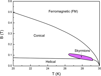
Figure 1. Temperature–magnetic field phase diagram of MnSi obtained through free energy minimization. Below the critical temperature of about 30 K, a helimagnetic ground state appears. As the applied magnetic field increases, it transforms into a conical phase and finally into a ferromagnetic state. Skyrmions appear in the form of crystal phase very close to Tc only in a tiny region of magnetic field and temperature.
Download figure:
Standard image High-resolution imageUsing the values of the equilibrium magnetization obtained from these phase diagram calculations, we can further calculate the magnetostriction strains at any given temperature and magnetic field through equation (4). Here, we chose the variation of Δε33 as an example, because it is easily measured experimentally. This quantity, Δε33 = ε33(b) − ε33(0), denotes the change of ε33 due to a change of the magnetic field.
The typical magnetic field dependence of Δε33 at the temperature T = 26.4 K is shown in figure 2(a). As the field increases from zero, the magnetostriction first decreases up to the lower critical field BC1 ≈ 0.07 T. It then increases approximately quadratically with the field strengthen up to the upper critical magnetic field BC2 ≈ 0.25 T. This is accompanied by a hill-like jump between the two fields BA1 ≈ 0.08 T and BA2 ≈ 0.11 T. At magnetic field higher than B > BC2, we obtain an approximately linear dependence of the magnetostriction on the field strength. Compared with the conventional magnetic phases in the prototypical helimagnet MnSi and in previous work [27], BC1 and BC2 are easily identified to correspond the critical fields for the helical-to-conical phase and the conical-to-ferromagnetic phase transition, respectively. The hill-like jump in the field range [BA1, BA2] characterizes the skyrmion phase.
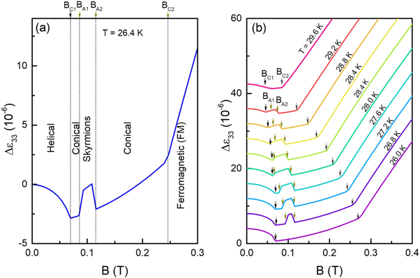
Figure 2. Variation of Δε33 with magnetic field, as obtained from theoretical calculations, at (a) 26.4 K and (b) different temperatures. The magnetostriction strains in the SkX phase are calculated using a fourth order Fourier representation of the SkX. Note that above about 28 K, the helical-conical phase transition is replaced by a helical-SkX phase transition, which is marked by BC1, while BA1 marks the conical-SkX phase transition and the conical phase is only metastable.
Download figure:
Standard image High-resolution imageThe detailed dependence of the magnetostriction on the magnetic field at various temperatures below Tc is shown in figure 2(b). This jumped behavior emerges in the whole region of the skyrmion phase.
3.1. Derivation of the analytical expression of magnetostriction strains in bulk MnSi
To explain this jump, we derive below analytical expression of magnetostriction strains for the SkX phase within the triple-Q approximation of the magnetization
with ![${{\bf{q}}}_{1}=q{\left[\begin{array}{lll}1 & 0 & 0\end{array}\right]}^{T}$](https://content.cld.iop.org/journals/1367-2630/21/12/123052/revision2/njpab5ec2ieqn30.gif) ,
, ![${{\bf{q}}}_{2}=q{\left[\begin{array}{lll}-\tfrac{1}{2} & \tfrac{\sqrt{3}}{2} & 0\end{array}\right]}^{{T}}$](https://content.cld.iop.org/journals/1367-2630/21/12/123052/revision2/njpab5ec2ieqn31.gif) ,
, ![${{\bf{q}}}_{3}=q{\left[\begin{array}{lll}-\tfrac{1}{2} & -\tfrac{\sqrt{3}}{2} & 0\end{array}\right]}^{T}$](https://content.cld.iop.org/journals/1367-2630/21/12/123052/revision2/njpab5ec2ieqn32.gif) , which yields from equation (4)
, which yields from equation (4)

For the conical phase, we have ![${{\bf{m}}}_{{\rm{conical}}}={\left[\begin{array}{lll}{m}_{{qc}}\cos \left({{qr}}_{3}\right) & {m}_{{qc}}\sin \left({{qr}}_{3}\right) & {m}_{0c}\end{array}\right]}^{T}$](https://content.cld.iop.org/journals/1367-2630/21/12/123052/revision2/njpab5ec2ieqn33.gif) ,which gives from equation (4)
,which gives from equation (4)
Comparing equations (6) and (7), we have

where it is found through calculation that m0 ≈ m0c and mq ≈ mqc, and the condition  ,
,  ,
,  ,
,  is used. The magnitude of the jump in ε33 through the phase transition from the conical phase to the SkX phase is determined by the coefficient
  . For MnSi
  , which yields the result in figure 2. Another phenomenon shown in figure 2(b) is that the jump in ε33 in the conical-skyrmion phase transition becomes more insignificant as the temperature rises. As shown in equation (6), the difference in ε33 between the SkX phase and the conical phase depends not only on the parameter
  but also on the value of mq. Since the skyrmion phase appears near the Curie temperature of the material, and near the Curie temperature we have
  , the difference of ε33 in the two phases gradually vanishes as the temperature rises. According to equation (7), this phenomenon is generally true for all strain components.
4. Experimental measurement of the magnetostriction strains in bulk MnSi
To test the theoretical results, we measured the magnetostriction of MnSi using the capacitance method [36]. We used a rectangular, single-crystal sample of MnSi that was 1.82 mm long, 1.09 mm wide, and 2.61 mm high, with the pair of end-faces parallel to the (001) crystallographic plane. We always measured the sample length in the [100] direction, which is also parallel to the orientation of the magnetic field.
The complete variation of Δε33 (calculated from ΔL/L, where L denotes the length in the height direction and ΔL denotes its variation) with the applied magnetic field for MnSi at different temperatures is shown in figure 3(a). The rules for defining the four critical points in figure 3(a) are as follows: BC1 denotes the field strength at which the first-order derivative dB/dT is zero; this corresponds to the minimum field in the low magnetic field region, which is marked by the black arrow in figure 3(b). The critical points BA1 and BA2 are defined as the maximum and minimum of the first-order derivative curve in the intermediate magnetic field region, as shown in figure 3(b). These two points define the region where skyrmions exist. The last transition field corresponds to an abrupt change in slope, as obviously shown by the sudden jump of ΔL/L in the derivative curve. This critical field BC2 in figure 3(a) is determined from the midpoint of the transition in d(ΔL/L)/dB, as marked by the black arrow in the derivative curve shown in figure 3(b). Figure 3(c) shows the experimental phase diagram for MnSi, which is constructed from figure 3(a).

Figure 3. (a) Variation of Δε33 with magnetic field. (b) The magnetostriction curve at 27.2 K and the corresponding first-order derivative curve, which is used to determine the four critical points and (c) The temperature–magnetic field phase diagram for MnSi obtained from experiments. (c) is obtained by extracting information from (a), where IM denotes an intermediate magnetic phase with strong fluctuations of magnetization and hence of the magnetostriction as well.
Download figure:
Standard image High-resolution image5. Discussion
We have shown that the experimental measurements well verified the theoretical results. The magnitude of the maximum jumped value of Δε33 is on the order of 2.5 × 10⁻⁷, the same as the theoretical result. Nevertheless, three discrepancies exist between experiment and theory. The first is that the jump in Δε33 between the magnetic phases is smoother in the experiment. The reason for this discrepancy is probably due to neglect of possible mixed states of the conical and SkX phases in the theoretical calculations. As shown by various TEM(Transmission Electron Microscopy) observations of the SkX phase [5, 6], at the critical magnetic field for the conical-SkX transition, some isolated skyrmions or skyrmion clusters appear due to the presence of defects or grain boundaries, thus forming a mixed state of conical and skyrmions phases, which smooths the jump in Δε33. The second concern is the intermediate magnetic (IM) state, which appears in a small window between the paramagnetic phase and the skyrmion phase in figure 3(c), but which is not present in the theoretical phase diagram shown in figure 1. In the IM phase, the magnetostriction strain changes smoothly, as illustrated by the curve for Δε33 at T = 29.6 K in figure 3(a), which indicates that the helical-conical transition is missing. This IM state may be related to the precursor states discussed in previous works [37–41] , but further exploration is needed to confirm this. The third concern is the phase transition at high temperature from calculated phase diagram is not consistent with the experimental one. The SkX phase is connecting to the helical phase at high temperature in theoretical calculation, but in experiment the SX phase is connecting to conical phase. This may be due to the fact that theoretical calculation is performed within mean-field approximation, where the effect of fluctuation is neglected.
6. Summary
In summary, we have derived a general expression of magnetostriction strains for B20 helimagnets in the SkX phase. For MnSi, we calculated the normal strain ε33 at different temperatures and magnetic fields, and we also perform the corresponding experimental measurements, which agrees quantitatively with each other. ε33 undergoes a sudden jump that accompany a conical-skyrmion phase transition at any temperature, which can be used to confirm the presence of the SkX phase.
Acknowledgments
This work was supported by the National Key R&D Program of China, grant no.2017YFA0303201, the Natural Science Foundation of China, grant no. 11772360, 51622105, the Key Research Program of Frontier Sciences, CAS, grant no. QYZDB-SSWSLH009, the Key Research Program of the Chinese Academy of Sciences, grant no. KJZDSWM01,Pearl River Nova Program of Guangzhou, grant no.201806010134.
: Appendix. Derivation of the rescaled free energy density functional incorporating magnetoelastic interactions
The free energy density functional for cubic helimagnets incorporating magnetoelastic interactions can be written as
where

and
Here ![${\bf{M}}={\left[{M}_{1},{M}_{2},{M}_{3}\right]}^{T}$](https://content.cld.iop.org/journals/1367-2630/21/12/123052/revision2/njpab5ec2ieqn42.gif) denotes the magnetization vector, Ms denotes the saturation magnetization, and
denotes the magnetization vector, Ms denotes the saturation magnetization, and  . The first term in equation (A.1) describes the exchange energy density with stiffness A; the second term is the Dzyaloshinskii–Moriya (DM) interaction with coupling constant D, which determines the period and direction of the periodic magnetization; the third term is the Zeeman energy density in the applied magnetic field B;
  are two Landau expansion terms; Ae denotes the coefficient of the exchange anisotropy; and wel and wme denote respectively the elastic energy density given in equation (A.2) and magnetoelastic free energy density given in equation (A.3).
Equation (A.1) provides an implicit model for studying the effects of magnetoelastic interactions on the SkX phase. The effects of these interactions cannot be understood by simply examining the magnetoelastic thermodynamic parameters, such as K, L1, etc., because they are also related to magnetic thermodynamic parameters, such as A and D. It is thus more convenient to write the free energy density functional in a rescaled form given in equation (A.1), where


and

The rescaled thermodynamic parameters (parameters with wavy overlines) are defined by

In equation (A.7),  , (i = 1, 2, ..., 6) can be derived from equation (A.4) by replacing M by m. In equation (7) of the main text, coefficients with the superscript '*' are defined by
Footnotes
- 4
The thermodynamic parameters of MnSi used in the calculation are presented in a rescaled form as
 , , , , , , , , , , . The original parameters can be found in [24].


