


Abstract
A new method to seamlessly simulate the continuous growth of droplets advected by turbulent flow inside a cumulus cloud was developed from first principle. A cubic box ascending with a mean updraft inside a cumulus cloud was introduced and the updraft velocity was self-consistently determined in such a way that the mean turbulent velocity within the box vanished. All the degrees of freedom of the cloud droplets and turbulence fields were numerically integrated. The box ascended quickly inside the cumulus cloud due to the updraft and the mean radius of the droplets grew from 10 to 24 μm for about 10 min. The turbulent flow tended to slow down the time evolutions of the updraft velocity, the box altitude and the mean cloud droplet radius. The size distribution of the cloud droplets in the updraft case was narrower than in the absence of the updraft. It was also found that the wavenumeber spectra of the variances of the temperature and water vapor mixing ratio were nearly constant in the low wavenumber range. The future development of the new method was argued.
Export citation and abstract BibTeX RIS

Original content from this work may be used under the terms of the Creative Commons Attribution 3.0 licence. Any further distribution of this work must maintain attribution to the author(s) and the title of the work, journal citation and DOI.
1. Introduction
Turbulence and cloud are key to understanding atmospheric dynamics, forecasting weather, and predicting the future climate. Because the minimum grid size in numerical weather (climate) predictions is of the order of a few kilometers under optimal conditions when using high performance computers, the degrees of freedom of turbulent flow and cloud microphysical processes, such as cloud condensation nucleation, condensation/evaporation, and collision/coalescence/breakup of water droplets below the grid size, are adequately modeled or parametrized with certain hypotheses. For example, both the bin and super droplet methods use the sub-grid model for the turbulent motion below the grid scale and the prescribed functional form for the collision kernel [1–6]. Although many efforts have been made to understand the dynamics of turbulence and cloud formation, and to develop more accurate models [1–9], our knowledge of these degrees of freedom is limited because turbulence is still not fully understood [10, 11], and the direct observation and measurement of cloud microphysical processes is difficult [12–15].
Then it is quite natural and reasonable to study the microphysical processes and turbulent transport from more fundamental view point according to first principle, which is to numerically compute all the degrees of motion as accurately with respect to the fundamental physics as possible. This approach requires both Eulerian and Lagrangian computations for the turbulence and the cloud droplets, respectively, and needs large computational resources. Recent progress in high performance computing has driven this trend. Vaillancourt, Yau, and Grabowski [16, 17] were the first to undertake this research for studying the broadening of the droplet spectrum (size distribution). They introduced a small parcel, which had a cubic domain of (15 cm)3 inside the quasi-adiabatic cloud core and derived two sets of equations for calculating the variables of the cloud and turbulent flow. A macroscopic set of equations was used to describe the evolution of the various means within the parcel, and a microscopic set of equations was used to describe the dynamics of each droplet and the turbulent fluctuations of velocity, temperature, and the water vapor mixing ratio. It was found that the increase in the variance of the droplet radius was too small to explain the observed broadening of the droplet spectrum by the sedimentation, randomness of the particle position and/or the initial variation of the droplet radius and turbulence.
Then droplet collision is considered to be a key process for the broadening of the droplet spectrum. The collision process of particles in turbulent flow, and its statistical properties, have been studied extensively since Saffman and Turner [18]. Many studies have analytically and numerically examined particle density [19, 20], collision frequency [21–24], and various influences on collision efficiency such as sedimentation [25–27], the clustering and spatial distribution of the inertial particles [28–36], and the hydrodynamic interaction [37–39]. It was found that the collision of cloud droplets with a similar size depends on the Stokes number  , where
  and
and  are the characteristic time of the droplet and the Kolmogorov time of turbulent flow, respectively, and becomes frequent for
  , at which the droplet radius is about 30 μm. Sedimentation due to gravity and the clustering of droplets with
  tends to enhance collisions.
However, these findings raise further questions, for example, as to how fast the cloud droplets grow from the water drops around the condensation nuclei to about 30 μm beyond which the collision/coalescence becomes important, how the size distribution of the aerosols affects the evolution of the droplet spectrum, and the condensation process in the supersaturated air dominates this early stage of growth but how can the supersaturated state be maintained? For the last question, a plausible way is to consider the adiabatic cooling by the updraft inside a cloud. However, at the same time the updraft engulfs the unsaturated air in the cloud and mixes it with saturated air and cloud droplets, the entrainment, which tends to slow down the droplet growth. Therefore, the updraft effects are not onefold but bring other factors into the droplet growth [40–50].
There are many accumulated knowledges for individual processes, but the whole is not necessarily a simple sum of elementary processes. What is necessary in the research for cloud evolution is a study that explores the continuous growth of cloud droplets from sub-micron to hundreds micron meter radius, a whole story of the rain drop formation. The goal of our research is to reconstruct the whole process, to elucidate the real feature of the phenomena and to extract the useful knowledge for better numerical modeling.
From the above arguments it is reasonable to infer a scenario about the rain drop formation that cloud droplets grow by condensation without an appreciable broadening of the droplet spectrum up to about 30 μm radius and then evolve into rain drops by the collision-coalescence. If this scenario is applied to the core region of cumulus cloud where the updraft exists, it suggests that the domain of the droplet growth dominated by the collision-coalescence is not necessarily the same as that dominated by the condensation. Therefore the computation of the cloud microphysics within a small domain fixed inside cloud as used in the previous studies is not appropriate for seamless computation of the continuous growth of the cloud droplets to the rain drops.
Our purpose in this paper is to present a new method that is able to seamlessly simulate the continuous growth of cloud droplets from about 10 μm to a few hundred μm with a minimum set of processes which are essential for the rain drop formation. And we examine its consistency from the view points of the numerical and physical properties. In order to study the evolution of the system in more natural and closer circumstances to the realistic conditions, we consider a scenario that a parcel which contains a large number of droplets and turbulence rises inside a typical maritime cumulative cloud as studied by Takahashi [51]. In the time domain, the evolution process to be studied is about 20 min. However, it should be stressed that in this paper we do not intend to accurately simulate all the processes in the cloud microphysics. Instead, we focus on to show effectiveness and wider capability of the new method for incorporating various detailed dynamics in the long time integration. As a first step, we studied the continuous growth, without collisions, of cloud droplets by condensation within a small parcel advected by the updraft. The paper is organized as follows. Section 2 describes the mathematical formulation of the problem, the equations of the fluid, temperature, the water vapor mixing ratio, and the droplets. Section 3 describes the direct numerical simulation (DNS) and the various numerical parameters. The results are presented in section 4, and the summary and discussions are given in section 5.
2. Fundamental equations
Here, we consider a small cubic box of length  which is moving with an updraft velocity
  inside a cumulus cloud above the tropical sea (see figure 1) [51]. The box contains many cloud droplets that undergo advection by turbulent flow and growth or decay due to condensation, evaporation or collision processes. A coordinate system
  whose origin is fixed on the sea surface is introduced in such a way that the z axis is set along the vertical upward direction and the x and y axes are in the horizontal directions. The environmental conditions for the cumulus cloud in this study are specified by the environmental temperature Te(z) and the environmental water vapor mixing ratio Qve(z), respectively. We assume that
  is much smaller than the typical length
  of the cumulus cloud. The turbulent velocity
  , temperature T, and water vapor mixing ratio Qv are well mixed on a scale larger than
  , but their fluctuations appear to be observable and statistically homogeneous (but axially symmetric) when seen on a scale below
  [42–47]. Therefore, it is reasonable to impose periodic boundary conditions in three directions for the three fields. We also assume that the fluid is incompressible and the buoyancy force is expressed in terms of the Boussinesq approximation. A local coordinate system
  is introduced in such a way that the system is attached to the cubic box and moves with the updraft
  . Two coordinate systems are related to each other by the time-dependent Galilean transform:

where  and
and  are the altitude of the box and the unit vector in the vertical direction, respectively. Then the equation of motion for the velocity field with respect to this coordinate is:

where  is the pressure,
  and
and  are the density and kinematic viscosity of dry air, respectively, and B is the buoyancy force which is given below. The updraft velocity
  is determined by the requirement that the volume average of the fluid velocity over the cubic box
  vanishes. Taking the volume average of the Navier–Stokes equation over
  and using the periodic boundary condition and the assumption
  , we obtain:

and

where the volume average is defined by:

With respect to this moving frame, the mean fluid velocity is zero so that the homogeneity of turbulent fields holds, but it should be noted that the mean velocity of the cloud droplets inside the box is not necessarily zero. The environmental temperature and water vapor mixing ratio at the altitude of the parcel are given by:


respectively. Note that the integration is made with respect to the z coordinate fixed to the sea surface. Here Te0 and Qve0 are the temperature and the water vapor mixing ratio of the environment at  , respectively, and
  and
and  are the lapse rate of the air and the rate of change of the water vapor mixing ratio
  , respectively.
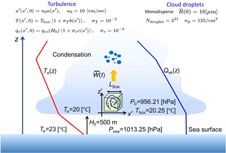
Figure 1. Coordinate system and initial conditions. The  and c are the multivariate Gaussian random numbers with the spectrum specified in section 3.
Download figure:
Standard image High-resolution imageThe incompressibility condition, the equations of the fluctuating turbulent velocity, the temperature T, and the water vapor mixing ratio Qv are given by:


respectively, where  is the external force that is introduced to maintain the turbulence in a steady state, the
  and
and  are the molecular diffusivity coefficients of the temperature and water vapor mixing ratio, respectively, Lv is the latent heat of vaporization, and cp is the specific heat of the air [1, 10]. The Cd is the condensation rate, which is discussed below, and the last term of the right-hand side of equation (10) denotes the adiabatic cooling due to the updraft and
  is the rate of change of the mean temperature inside the parcel at
  which is described below. Because the box size
  is much smaller than the cloud size, the contributions from the vertical fluctuating fluid velocity
  to the adiabatic cooling is neglected. The
  is assumed to be given by the sum of two contributions as


where  is the effect of the moist air and
  is the dry adiabatic lapse rate. When the parcel is ascending, the moist air is very close to being supersaturated (
 ) and when it is descending the parcel of air is undersaturated (
 ). The
  is the effect due to the entrainment [1, 2] and μ is the entrainment strength parameter.
For the cloud droplets, we followed the formalism developed by Vaillancourt, Yau and Grabowski [16]. The microscopic dynamics of the cloud droplets are assumed to be specified by the position  , the velocity
  , and the radius Rj(t) of the jth droplet, with respect to the comoving frame. Then, the buoyancy force
  , the condensation rate
  , and the liquid water mixing ratio
  , are given by


where g is the gravitational acceleration, and  , where Rd and Rv are the gas constants for dry air and water vapor, respectively.
  is the number of droplets within the grid cell
  ,
,  is the liquid density, respectively, S is the supersaturation, and Ks is a temperature-dependent diffusion coefficient specified below.
The cloud droplets are assumed to move around inside the box under the turbulence, the gravity force and the Stokes drag. The use of the Stokes drag for the cloud droplet is justified for droplets with a radius smaller than 30 μm in this study because the droplet Reynolds number is smaller than unity. Then, the equations of motion of the cloud droplets with respect to the comoving frame are:


where  and
and  are the relaxation time and the supersaturation at the particle position defined by


respectively, and:

where  is the saturated vapor density. We assume that the supersaturated water vapor mixing ratio Qvs at the droplet position is determined by Tetens' formula:

The pressure and the altitude are related by:

where  is the pressure at the sea level and set to be 1013.25 (hPa).
3. DNS of cloud droplets and turbulent flow
The set of equations (8)–(25) is numerically integrated over about 20 min. For cloud droplets with a radius of the order of 10 μm the representative time increment  is about 1 ms, and therefore the total number of time steps for one run is 1.2 million, which requires long time integration and large computational resources. Before proceeding to heavy computations it is important to examine the consistency of the above microscopic equations with the macroscopic behavior that has been found by many previous studies. Also knowing in advance the average behavior of the above microscopic equations is helpful and useful to choose proper parameters for DNSs of the full set of equations such as the environmental temperature, entrainment strength, and so on. For this purpose, we studied a parcel model which is obtained by taking the volume average of the equations derived in the previous section and described in detail in the
The equations under consideration are equations (8)–(17) for the turbulent air flow, equations (18)–(25) for the droplets. The numerical methods used were as follows. For the spatial derivatives, we used a hybrid code, which employs the spectral method for the velocity field and the combined compact finite difference method (CCFD) for the temperature and the water vapor mixing ratio. We developed an efficient three-dimensional fast Fourier transform (3DFFT) using the two-dimensional domain decomposition, and we also developed an efficient solver for the 8th order CCFD using a three-dimensional domain decomposition. The numerical accuracy and performance of the hybrid code have been carefully examined in [52] and were found to be very satisfactory. The velocity and scalar fields at the droplet position were linearly interpolated, and the contributions from the condensation term and the buoyancy force were distributed on the surrounding grid points using the same weighting as that of the linear interpolation, i.e., the particle in the cell method (PIC). The time integration was made in terms of the predictor corrector method.
The environmental temperature and water vapor mixing ratio in the air are taken from observation data at Hawaii [51] and approximately given by

and

where  and the argument z of
  of equation (6) and
  of equation (7) is now switched to the pressure P as
  and
and  using equation (25) as is often used. Note that
  and P0 is the pressure at
  , the initial position of the box. The distributions of Te(P) (red, color online) and Qve(P) (blue) are plotted in figure 2 as functions of the pressure (left axis) as well as functions of the altitude (right axis). It is seen that the inversion occurs at 780 hPa (about 2200 m above the sea surface).
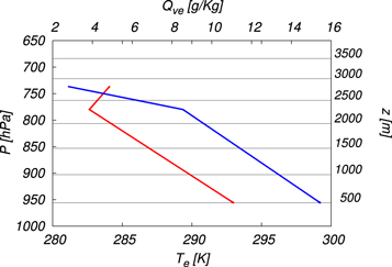
Figure 2. Environmental temperature Te(P) (red, color online, bottom axis) and water vapor mixing ratio Qve(p) (blue, top axis) [51]. The left axis is the pressure and the right axis is the altitude corresponding to the pressure.
Download figure:
Standard image High-resolution imageA cubic box with size  is initially at rest
  ms−1 at
  , at which the mean temperature and mean water vapor mixing ratio in the environment are:

respectively. Inside the box, the mean temperature is set to be slightly higher than the environmental temperature as:

The mean water vapor mixing ratio is assumed to be saturated and is determined by Tetens' formula for the saturated vapor pressure as:

and then the mean water vapor mixing ratio is:

The Ks, which is defined by equation (23) and used in equation (16), was treated as a constant determined by T0 and P0 for most runs because the temperature dependence was found to be very weak. The entrainment strength μ in (14) is chosen to be  cm−1.
cm−1.
The fluctuating turbulent velocity  and the fluctuations of temperature θ and water vapor mixing ratio qv are defined as follows:

The fluctuations are assumed to obey multivariate Gaussian statistics with zero means. The kinetic energy spectrum and the variance spectra of the temperature and water vapor mixing ratio are defined by:


respectively, where  is the ensemble average and
  and q0 are the root mean square velocity, temperature, and water vapor mixing ratio, respectively. The initial kinetic energy spectrum is:

where k0 is the peak wavenumber and is set to be  and
and  cms−1. The spectra
  and
and  are of the same functional form as equation (36), with amplitudes of
  and
and  , respectively.
The cloud droplets are assumed to be monodisperse, with an identical radius of 10 μm and are uniformly distributed inside the box, with zero initial velocity. The mean number density of the droplets np is 125 cm−3, which is a typical value in a cloud. Various parameters are summarized in table 1.
Table 1. Various parameters. Np and np are the total number and the mean number density of droplets, respectively.
| Box length |

|
25.6 (cm) |
| Number of droplets | Np | 221 |
| Droplet number density | np | 125 (cm−3) |
| Initial temperature at 500 m | Te0 | 293 (K) |
| Pressure at sea surface |
 |
1013.25 (hPa) |
| Gas constant of dry air | Rd |
 (cm2 s−2 K−1) (cm2 s−2 K−1) |
| Gas constant of water vapor | Rv |
 (cm2 s−2 K−1) (cm2 s−2 K−1) |
| Specific heat for constant pressure | cp |
 (cm2 s−2 K−1) (cm2 s−2 K−1) |
| Dry adiabatic lapse rate |

|
 (K cm−1) (K cm−1) |
| Latent heat of vaporization | Lv |
 (cm2 s−2) (cm2 s−2) |
| Initial saturated vapor pressure |

|
 (g cm−1 s−2) (g cm−1 s−2) |
| Density of saturated water vapor |

|
 (g cm−3) (g cm−3) |
| Density of dry air |

|
 (g cm−3) (g cm−3) |
| Kinematic viscosity of dry air |

|
 (cm2 s−1) (cm2 s−1) |
| Thermal diffusivity |

|
 (cm2 s−1) (cm2 s−1) |
| Diffusivity of water vapor |

|
 (cm2 s−1) (cm2 s−1) |
In this computation, the buoyancy force is not strong enough to maintain the turbulence in a statistically steady state and random force is applied to the turbulence. The solenoidal random force is assumed to be a Gaussian random with zero mean and to be white noise [55]. It is applied to the low wavenumber band as:

where  and F(k) is the spectrum of the random force and is given by:

where cf is a constant and is set to be 70 cm2s−3.
The turbulence in the box is statistically homogeneous and axially symmetric due to the buoyancy force in the vertical direction. Therefore, it is reasonable to expand the statistical quantities in terms of the Legendre polynomials [56]. However, we consider only the zeroth order coefficients (i.e., the isotropic parts) for simplicity of analysis. The integral scale, Taylor microscale and the Taylor microscale Reynolds number are defined by:

respectively, and the rate of kinetic energy dissipation per unit mass and the mean Kolmogorov length of the turbulent flow are defined by:

respectively.
The target range of time evolution for the present DNS is about 20 min and the total number of time steps with the time increment  1 ms is 1.2 million. Therefore, we examine the small system with the grid number
  as the first step in future large-scale computations. Five computations were made and the numerical and turbulence parameters are summarized in table 2. Runs 1, 2, 3a, and 4 used four different values of μ to examine the entrainment effects. Run 3b was made using
  to compare with the case of zero updraft. The computers used were the K-computer at the Research Organization for Information Science and Technology in Kobe and the FX10 at Nagoya University and the University of Tokyo.
Table 2.
Numerical and mean turbulence parameters. Updraft is On for  , Off for
  . μ is the entrainment strength.
| Updraft | μ |

|
E |  |

|
λ | η | |
|---|---|---|---|---|---|---|---|---|
| ×10−5 (cm−1) | (cm2 s−2) | (cm2 s−3) | (cm) | (cm) | (cm) | |||
| Run 1 | On | 2.5 | 86 | 73.3 | 32.5 | 5.58 | 1.84 | 0.101 |
| Run 2 | On | 5.0 | 86 | 73.8 | 33.0 | 5.58 | 1.84 | 0.101 |
| Run 3a | On | 7.5 | 86 | 73.6 | 32.8 | 5.58 | 1.84 | 0.101 |
| Run 3b | Off | 7.5 | 86 | 73.6 | 32.8 | 5.58 | 1.84 | 0.101 |
| Run 4 | On | 10.0 | 86 | 73.3 | 32.8 | 5.58 | 1.84 | 0.101 |
4. Results
4.1. Mean values
Figures 3 and 4 show the time evolution of the mean updraft velocity  and the altitude
  of the parcel for Run 3a (red, color online), respectively. Also the curves of the parcel model (green) are plotted to see the turbulence effects. The
  attains a maximum of about 8 ms−1, and
  quickly reaches 2500 m at about 600 s and then slowly increases in time with the oscillation, which are compared to the results of 2.5 ms−1 at 5 min and 7.7 ms−1 at 25 min that were obtained by the bin method in Takahashi [51]. The period of oscillation is about 330 s which is longer than 310 s for the parcel model and about 50% longer than the Brunt Väisälä period that is about 220 s. This deviation is reasonable when considering the difference between the linear stability analysis and the fully nonlinear computation. The difference between the DNS and the parcel model in figures 3 and 4 is due to the fluctuations of the temperature, the water vapor mixing ratio and the droplets radius generated by the turbulent motion. The turbulence tends to slow down the evolution of
  and
and  and to slightly decrease the oscillation amplitudes. Figure 5 shows the time evolution of the mean temperature
  (red, color online) inside the parcel and that of the environment (blue, color online) at the same altitude as that of the parcel for Run 3a. When the parcel ascends,
  decreases below the environmental temperature and increases according to the parcel'(s) descent, and then begins to oscillate. The time evolution of the mean water vapor mixing ratio is similar to that of the mean temperature, but is always larger than the environmental value (figure not shown). Figure 6 indicates the time evolution of each component (temperature BT, water vapor mixing ratio Bq, and the liquid water mixing ratio Bql) and the total buoyancy force B for Run 3a. It can be seen that the temperature term dominates the buoyancy force and the liquid water mixing ratio becomes comparable to the temperature variation at later times due to the growth of the cloud droplets. The water vapor mixing ratio makes a small contribution.

Figure 3. Time evolution of  . Red:Run 3a; green: parcel model.
Download figure:
Standard image High-resolution image
Figure 4. Time evolution of  . Red: Run 3a; green: parcel model.
Download figure:
Standard image High-resolution image
Figure 5. Time evolution of  inside the box (red) and the temperature of the environment at the same altitude as that of the parcel (blue) for Run 3a.
Download figure:
Standard image High-resolution image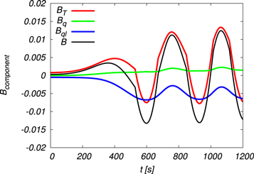
Figure 6. Time evolution of each term of the buoyancy force and total buoyancy force for Run 3a.
Download figure:
Standard image High-resolution image4.2. Turbulent flow
Now we consider the evolution of the turbulent flow inside the parcel. To examine the updraft effects, we compare Run 3a for  with Run 3b for
  . However, the differences in the one point statistics of the fluctuating velocity and temperature,
  and Eθ are very small for the two cases. Therefore, we describe the updraft effects for the cases when they are appreciable.
Figures 7 and 8 show the time evolution of  and
and  for Run 3a, respectively. The turbulent flow is in a statistically steady state and
  fluctuates around the mean value of 86 during the computation and the time averaged kinetic energy dissipation rate per unit mass
  is 33 cm2 s−3. These values mean that the turbulence in this study is very weak when compared to the values in the actual cloud because of the computational limitation. The updraft effects are seen in Eq(t) as shown in figures 9 and 10 for Runs 3a and 3b, respectively. The fluctuation amplitude of Eq(t) for Run 3a is slightly suppressed when compared to the case in the absence of the updraft. This is because the water vapor is more systematically condensed on the droplets when the supersaturated state is maintained by the adiabatic cooling due to the updraft. At times after t = 600 s Eq(t) begins to oscillate and its fluctuation amplitude increases when the parcel is close to the local minimum or maximum altitude.
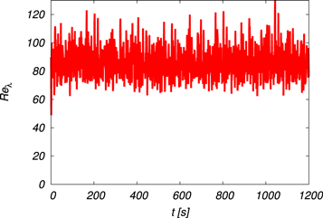
Figure 7. Time evolution of  for Run 3a.
Download figure:
Standard image High-resolution image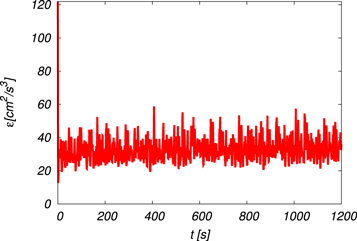
Figure 8. Time evolution of  for Run 3a.
Download figure:
Standard image High-resolution image
Figure 9. Time evolution of Eq(t) for Run 3a.
Download figure:
Standard image High-resolution image
Figure 10. Time evolution of Eq(t) for Run 3b.
Download figure:
Standard image High-resolution imageAlthough the updraft effects on the one point statistics are appreciable only in the water vapor, the spectrum is more sensitive to the updraft. Figures 11–13 show the time variation of three spectra  , and
, and  for Runs 3a and 3b at 760 s (red), 770 s (green), 840 s (blue), 890 s (magenta), 920 s (cyan), 930 s (black). As for the kinetic energy spectrum, there is almost no difference in
  . This is because (1) the mean buoyancy force (which corresponds to the Fourier mode at the origin,
  ) generating the uniform updraft is subtracted from the buoyancy force as
  so that no direct effects of the updraft can be observed in the turbulence and (2) the amplitude of the buoyancy force is smaller by about two order in magnitude than the random force and masked by the random force. On the other hand,
  and
and  are affected by the updraft. They are approximately constant at
  and oscillate in time. By comparing the time variation of these spectra with
  in figure 4, we see that the one period of the oscillation of the spectra roughly corresponds to the half the oscillation period of the parcel altitude. However, this correspondence becomes obscure at latter times. The condensation term
  acts as the source of the scalar fluctuations at scales smaller than the Kolmogorov scale (note that Sc = 0.72 so that
  , where
  is the Batchelor length). The fluctuations of the water vapor and temperature generated by
  are advected by the turbulent flow and spread over the entire domain of the box. In the wavenumber space, the excitation of
  at high wavenumbers (figure not shown) is quickly transferred toward the low wavenumbers and begins to oscillate in time. The same mechanism can be applied to
  and
and  but without oscillation when the updraft is absent as seen in figures 12(b) and 13(b).
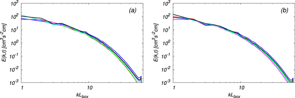
Figure 11. Time evolution of  . (a) Run 3a, (b) Run 3b.
  (red), 770 s (green), 840 s (blue), 890 s (magenta), 920 s (cyan), 930 s (black).
Download figure:
Standard image High-resolution image
Figure 12. Time evolution of  . (a) Run 3a, (b) Run 3b.
  (red), 770 s (green), 840 s (blue), 890 s (magenta), 920 s (cyan), 930 s (black).
Download figure:
Standard image High-resolution image
Figure 13. Time evolution of  . (a) Run 3a, (b) Run 3b.
  (red), 770 s (green), 840 s (blue), 890 s (magenta), 920 s (cyan), 930 s (black).
Download figure:
Standard image High-resolution imageThe spectra  and
and  have quite large cusps near the high wavenumber cut off, which is in sharp contrast to
  . The cusp has two origins: the first is due to the fact that the fluctuations are injected at small scales below the computational grids, while the second is due to the fact that the contributions of Cd are treated as the point force. This behavior has also been observed and is unavoidable—in the DNS, which used the point particle approximation to the droplet [22]. It is difficult to make a quantitative assessment of the two contributions, and therefore we do not consider this problem further.
4.3. Cloud droplets
Figures 14 and 15 show a comparison of the time evolution of the mean droplet radius and the variance of the droplet radius around the mean for Run 3a (red: color online) and Run 3b (blue), respectively. Also the result of the parcel model is plotted in figure 14 for comparison. The effects of the updraft are very dramatic when compared to the case with no updraft. Starting from 10 μm the  grows to about 24 μm by 600 s at which
  and begins to oscillate according to the parcel oscillation at the inversion layer. This result is not far from the data of 30 μm at 2000 m above the sea as reported in [51]. Although the oscillation amplitude gradually decreases, the maximum of
  remains almost unchanged. In contrast, the
  for the zero updraft case grows very slowly. When compared to the parcel model, the turbulence tends to make the evolution slower and to decrease the oscillation amplitudes.

Figure 14. Time evolution of  . Red: Run 3a; blue: Run 3b; green: parcel model.
Download figure:
Standard image High-resolution imageThe evolution of the distribution of the cloud droplet radius is a main target of the present simulation. Figure 15 shows the comparison of the evolution of the variance of the droplet radius fluctuations for Runs 3a and 3b. It is interesting to observe that the variance for Run 3a becomes smaller than that for Run 3b. This is because all the droplets grow uniformly in the box due to the decrease of the saturated vapor pressure when the parcel ascends. Figures 16(a) and (b) show the time evolution of the droplet spectrum for Runs 3a and 3b, respectively. The peak of the droplet spectrum for Run 3a moves rapidly to the right with increase of time and then oscillates at around 20 μm, while the droplet spectrum for Run 3b moves slightly to the right and the spectrum width is a little wider than that for Run 3a, which is consistent with figure 15.
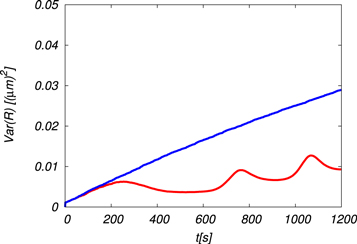
Figure 15. Time evolution of the variance of cloud droplet radius. Red: Run 3a; blue: Run 3b.
Download figure:
Standard image High-resolution image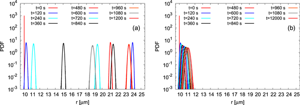
Figure 16. Time evolution of droplet spectrum. (a) Run 3a, (b) Run 3b.
Download figure:
Standard image High-resolution imageFigure 17 indicates comparison of the time evolution of the liquid water content (LWC), which is defined by:

When compared to the parcel model (green) the LWC by the DNS (red) increases slowly and begins to oscillate around 5 gm−3, which is consistent with the value observed in the cloud. Figure 18 shows the variation of the mean vertical velocity of the cloud droplets with respect to the moving parcel frame. When the updraft exists, the mean vertical velocity is negative at all times and the amplitude slowly increases, and then begins to oscillate between about −8 and −4 cm s−1, which means that the cloud droplets are slowly falling inside the parcel. However, because the mean updraft velocity is oscillating between about 8 ms and −6 ms−1, the ensemble of cloud droplets is, as a whole, comoving with the parcel. The droplet Reynolds number, based on the mean droplet vertical velocity with respect to the air inside the parcel, is about 0.2, and therefore the use of Stokes' law for the droplet drag in this study is justified.
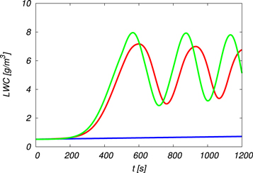
Figure 17. Time evolution of liquid water content. Red: Run 3a; blue: Run 3b; green: parcel model.
Download figure:
Standard image High-resolution image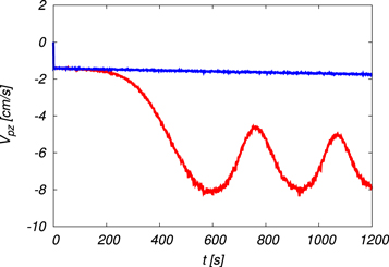
Figure 18. Time evolution of the mean vertical velocity of cloud droplets. Red: Run 3a; blue: Run 3b.
Download figure:
Standard image High-resolution imageIt is well known and discussed in the literature that the entrainment affects the evolution of the updraft velocity and the parcel altitude, which in turn leads to different evolution history of droplets inside the parcel [3]. Since the parcel is assumed to be small and advected inside the whole cloud, unlike the LES model, the entrainment strength can not be determined within the present microscopic approach but is given as the parameter [40–50]. Then it is useful and necessary for the future development of the present method and for large scale computations at very high Reynolds numbers with larger box size to know the variation of the above results to change of the entrainment strength. Different entrainment strength may, roughly speaking, be considered to be the difference in the initial position of the parcel, core region for low μ and near interface region between cloud and clear air for high μ [3].
We performed four computations Runs 1, 2, 3a, and 4 by changing μ while keeping other parameters the same, and these are summarized in table 2. Although these values of μ are larger than the values, for example, those between  and
and  used in [53, 54], they were chosen partially by the reason for the numerical stability. Since our main purpose in the present study is to examine the consistency of the new method, we do not enter the detailed arguments for the parameter. The effects of the entrainment on the parcel altitude and the mean droplet radius are compared in figures 19 and 20, respectively. The general trend is that when the entrainment μ decreases the oscillation amplitudes become larger and the oscillation period becomes gradually shorter and the migration of the mean parcel altitude tends to be higher. This trend is observed also in
  and the LWC (figure not shown) and is consistent with the previous studies [57–60].

Figure 19. Comparison of  for various strengths of entrainment.
Download figure:
Standard image High-resolution image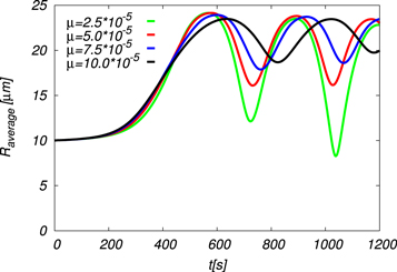
Figure 20. Comparison of  for various strengths of entrainment.
Download figure:
Standard image High-resolution image
Finally, we examined the effects of the temperature dependence of the diffusion constant Ks on cloud droplet growth. However, the effects on the mean radius of the cloud droplets were found to be very weak in this study.
5. Summary and discussions
We have developed a new numerical method that simulates the detailed dynamics of cloud droplets from the microscopic view point. Novel feature of the present method is the introduction of the parcel advected by the updraft that is self-consistently determined within the theory, so that the seamless computation for the continuous growth of the droplets along the parcel trajectory inside the cloud becomes possible. We call the set of equations of motion and growth of the radius of a large number of cloud droplets, and the equations of turbulent flow, temperature, and water vapor mixing ratio as the cloud microphysics simulator.
Continuous evolution of the droplets and turbulence during 20 min has successfully been simulated by the cloud microphysics simulator which has previously not been possible in simulations resolving all the degrees of freedom of cloud droplets. By the seamless simulation we found that (1) the mean radius of the cloud droplets grows from 10 μm to about 24 μm, (2) the turbulence slows down the evolution of the system when compared to the prediction by the parcel model, and (3) the width of the droplet spectrum becomes narrower than that in the absence of the updraft.
It is worthwhile and important to examine the effects of fluctuations due to the turbulence. In the parcel model all the droplets are assumed to be exposed to the same supersaturation and have the same radius and the same condensation rate, which leads to a systematic build up of the buoyancy force. On the other hand, the turbulent flow advects the droplets, temperature and water vapor so that the particle positions and radii change randomly in space and time. These fluctuations prevent the buoyancy force that is uniform inside the box from building up, as a result the evolution of the mean  becomes slower than in the case of the parcel model, and so do for the means of
  and
and  . This is the reason for the slow down of the mean evolution of the cloud droplets by turbulence although the effects are small for the case of the condensation alone. When the collision-coalescence is included, the effects of turbulence would become stronger because the variation of the mean and fluctuations of
  become larger. It should be noted that the total water mass (
![$M(t)=\int [{M}_{{\rm{d}}}{Q}_{{\rm{v}}}({\boldsymbol{x}},t)+{q}_{{\rm{l}}}({\boldsymbol{x}},t)]{\rm{d}}{\boldsymbol{x}}$](https://content.cld.iop.org/journals/1367-2630/18/4/043042/revision1/njpaa215aieqn164.gif) where Md is the mass of dry air inside the parcel) is conserved (indeed, it was numerically conserved within 0.2% accuracy) in the present set up even when the collision coalescence is included.
where Md is the mass of dry air inside the parcel) is conserved (indeed, it was numerically conserved within 0.2% accuracy) in the present set up even when the collision coalescence is included.
In the present study, the updraft generated by the mean buoyancy force is treated as a time dependent uniform flow in the vertical direction which can only indirectly drive the turbulence through the variation of the parcel height. When a whole cloud is considered, there exists non-uniformity of the updraft and the large scale shear appears as driving force to the turbulence. Since the parcel size is so small when compared to the whole cloud, such a mechanism is not incorporated within the present framework and must be introduced as the external force. The random external force in this study was weak in the sense that  was very small when compared to the one observed in the cloud, which is of the order of 103, but quite strong to mask the effects of the buoyancy force
  . The dominance of the random force over the buoyancy force is due to the artificial nature of the white in time property. In the future study a random force with finite memory should be considered [3].
Since the detailed dynamics of the cloud droplets are naturally incorporated in the cloud microphysics simulator, the process of collision-coalescence of the droplets with effects such as the offset distance, the relative droplet sizes, the surface tension, the Reynolds number dependence of the drag, and the hydrodynamic interaction are to be examined. Also the DNS of turbulent flow with a large number of grid points and cloud droplets is required to study the early phase of formation of rain drops and cloud. To conclude the cloud microphysics simulator developed in this study is very successful and promising. Its application to the above issues and further developments are great challenges in turbulence and cloud physics research.
Acknowledgments
The authors thank Prof. Watanabe for his valuable discussions and comments. This research used the computational resources of the K computer provided by the RIKEN Advanced Institute for Computational Science, through the High Performance Computing Infrastructure (HPCI) System Research project (hp120147, hp140024, hp150088). The computational support provided by Japan High Performance Computing and Networking, Large-scale Data Analyzing and Information Systems (JHPCN) (jh130010, jh140025, jh150012), and High Performance Computing (HPC) at Nagoya University are also appreciated. TG was supported by Grants-in-Aid for Scientific Research Nos.15H02218 and 24360068, and IS by No. 15H02218, respectively, from the Ministry of Education, Culture, Sports, Science, and Technology of Japan.
Appendix
Parcel model is a set of equations of means constructed by taking the volume average of the equations derived in section 2. Then all of the spatial derivative terms of equations (9)–(11) vanish by the periodic boundary condition. Replacing the average of the product of the fluctuating quantities by the product of their means, we obtain the parcel model as:


where


where  is given by equations (12)–(14). The numerical computations were made for the same constants, and the same initial and environmental conditions as those in DNS with various entrainment strengths. The results for the entrainment strength
  are plotted in the green lines in figures 3, 4, 14 and 17.
Equations (42)–(45) are the same as equations (11)–(15) of [16] for the macroscopic variables, although the precise meaning of 'macroscopic' is not given in their derivation. In our derivation, the volume average is defined in equation (5) and the mean values correspond to their macroscopic variables. The differences are: (1) the updraft velocity  in [16] is constant and given as parameters and the buoyancy force is dropped, while in the present study it is self-consistently determined through the buoyancy force term; (2) the saturation vapor pressure is given as a function of the altitude using Tetens' formula, but it is not certain whether or not it is constant in [16]; (3) Te and Qve are taken from the observation data of [51], while they are treated as constants in [16]; (4)
  has two contributions from the effects of the moist air and the entrainment, while it is a constant in [16].