
Abstract
High-speed plasma plays an important role in diverse areas. Plasma flow with a sufficiently high speed to arouse compression is usually not in thermal equilibrium, and the plasma characteristics are closely coupled with the flow field. The relation between the flow and the plasma parameters, especially the distributions of electron density, i.e. ne, and the electron temperature, i.e. Te, are of ultimate importance; however, this is not yet completely understood. In this work, a weakly compressible plasma jet produced by an arc torch is diagnosed using a Langmuir triple probe. The two-dimensional distributions of ne and Te are obtained consisting of 80 spatial points under arc currents of 70–100 A. The spatial patterns of the distributions demonstrate alternative expansion–compression wave structures. As the arc power increases, the wave structures remain almost unchanged, while ne increases monotonically. Moreover, in some regions Te decreases with the arc power, which has seldom been reported in the literature. In addition, the peaks of the radial distributions of Te always deviate from the central axis. These results are compared with previous works of strongly compressible plasma flows. The phenomena are then analyzed and explained from the perspective of fluid wave-plasma interactions and the actions of the ambipolar field in the electrons.
Export citation and abstract BibTeX RIS

Original content from this work may be used under the terms of the Creative Commons Attribution 4.0 licence. Any further distribution of this work must maintain attribution to the author(s) and the title of the work, journal citation and DOI.
Nomenclature
| d0 | Anode exit diameter |
| Di, De | Diffusion coefficients for ions and electrons, respectively |
| DC | Direct current |
| e | Electron charge quantity |
| E | Biased voltage in triple probe |
| Ekinetic | Kinetic energy of the electrons per unit volume |

| Electric field |
| EEDF | Electron energy distribution function |
| f | Electron velocity distribution function |
| I | Probe current or arc current |
| kB | Boltzmann constant |
| LTE | Local thermal equilibrium |
| mi, me | Ion mass and electron mass, respectively |
| ne | Electron density |
| ng | Ground-state atom density |
| nm | Metastable atom density |
| nt | Total heavy particle density, i.e. ne + nm + ng |
| pe | Electron pressure |
| Qgi | Reaction rate coefficient of electron-impact ionization of ground state atoms |
| Qgm | Reaction rate coefficient of electron-impact excitation from ground state to metastable state |
| Qig | Reaction rate coefficient of radiative recombination |
| Qmg | Reaction rate coefficient of electron-impact quench of metastable atoms |
| Qmi | Reaction rate coefficient of electron-impact ionization of metastable atoms |
| Qtri | Reaction rate coefficient of three body recombination |
| r | Radial position |
| R | Electric resistor or reaction rate |
| S | Collecting area of each probe pin |
| t | Time |
| Te | Electron temperature |
| U | Voltage |

| Velocity |
| v | Velocity magnitude |
| z | Axial position |
| σi | Ionization cross section |
| Φ | Electric potential |
| ξe, ξm | Density ratios of electrons and metastable atoms to total heavy particle density, respectively |
| μi, μe | Mobilities for ions and electrons, respectively |
| δ | Variational operator (math.) |
1. Introduction
High-speed plasma flow has attracted an increasing amount of interest for its versatile applications in a large number of areas, such as plasma spraying in material processing [1–3], electric propulsion [4–8] and flight simulations in high-velocity rarefied wind tunnels [9–11]. Within the plasma flow, ne and Te are critical parameters, since most concerned issues are directly related to them, such as thermal radiation, which is highly affected by Te and has a cubic increasing relation with ne [12, 13]. In addition, the relation between ne and Te, like Saha equation which is used for calculating thermodynamic properties and transport coefficients, is also important in theoretical analysis and numerical study.
However, in high-speed plasmas, thermal nonequilibrium can occur [14] which breaks the rule of the Saha equation. Due to the thermal nonequilibrium, it is extremely difficult to establish a general relationship, such as the Saha equation between ne and Te for high-speed plasmas, although there have been attempts [15–18]. Hence, the experimental diagnosis of nonequilibrium plasma is usually used to determine ne and Te, and subsequently their relationship, for specific conditions. The diagnosis results not only serve a specific purpose, but also provide evidence for the theoretical analysis and theoretical development of nonequilibrium plasma and serve as a reference for numerical study and empirical relation verification.
There have been many experimental diagnoses on high-speed plasmas using methods based on electrostatic probes [19, 20], optical emission spectroscopy [21], laser induced fluorescence [22, 23] and laser scattering [24–26]. In particular, D C Schram's group conducted a very detailed diagnosis on a cascaded arc torch using Thomson–Rayleigh scattering [24, 25] and laser induced fluorescence [23] methods. A scaling law agreed well with the diagnosis results [23]:

where n and z represents the number density of the electrons or the heavy particles and the axial position n0 and d0 are the values near the exit and the radius of the arc channel of the torch, respectively. Moreover, they proposed another scaling law [27]:

where χ and C0 are positive scaling parameters and could be derived from fitting the experimental data. The relation of equation (2) fitted the axial distributing data well, as shown in [27].
Nevertheless, those scaling laws were based on the adiabatic assumption [23–25], so they might not be able to predict the electron behaviors where the adiabatic assumption is not suitable, such as where the flow velocity is not supersonic and the time scale consideration is long enough for heat exchanges. Therefore, more experimental research is still needed.
In this article, we report on the experimental diagnosis of the two-dimensional spatial distribution of ne and Te within a sonic/subsonic high-speed plasma jet, which is produced by a direct current non-transfer arc torch under a reduced pressure. The relationship between the electron density and the electron temperature, as well as its response with the variations of the input powers, are analyzed, and the results are compared with those of supersonic plasmas.
Electrostatic triple probes are used for diagnosis for the sake of spatial resolvability and easy implementation. The theory of the probe is based on three assumptions [28]:
- (a)The electron in the sheath is collisionless;
- (b)The ion sheath thickness is small compared with the separation of each probe in the triple probe;
- (c)The electrons in the plasma obey a Maxwellian energy distribution.
Under the experimental conditions, the mean free path length of the electron and the Debye length are approximately 0.1–1.0 mm and 10−6 m, respectively, and the separation of the probes is 2 mm, which satisfies the requests of (1) and (2). Typically, the last assumption is widely accepted in the study of high-speed plasmas [18, 29–31], where the electrons and heavy particles have different temperatures, but the electron energy distribution function (abbr. EEDF) is considered as Maxwellian, as in the two-temperature model [32–35].
2. Experiment method
2.1. Experiment setup
The plasma jet was produced using a non-transfer direct-current arc torch with a long interelectrode, as schematically shown in figure 1. The torch is mainly composed of a cathode, two electrically isolated inter-electrodes, and an abruptly expanding anode. The main features of the torch are the relative steadiness due to the fixed length of the arc column and the relatively large and uniform plasma area of the plasma jet. Further information about the structures and characteristics of the torch is provided in [36].
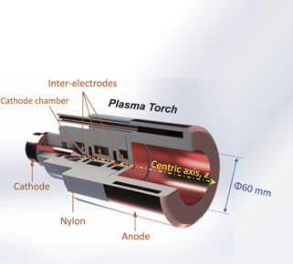
Figure 1. Schematic diagram of the plasma torch with a long inter-electrode channel and an abruptly expanded anode.
Download figure:
Standard image High-resolution imageExperiments were conducted in a vacuum chamber with dimensions of Φ1.3 m × 0.45 m. The background pressure was kept at approximately 200 Pa during the experiments. Pure argon was fed with a flow rate of 8.5 slm (standard liter per minute). Under this flow rate, the I–V curve of the torch is shown in figure 2 with an arc current varying from 70 A to 120 A, corresponding to the input power ranging from 5 kW to 8 kW. Fluctuations of the torch were highly suppressed [36], and the arc voltage variations, which were due to the Helmholtz oscillation, were approximately 4% of the mean voltage [37] in the range of the working conditions. Since the Helmholtz oscillation is high-frequency and has a small amplitude, the plasma jet is quasi-steady.
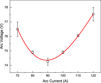
Figure 2. The I–V characteristics of the torch under the experiment condition.
Download figure:
Standard image High-resolution image2.2. The electrostatic triple probe
The Langmuir triple probe used in the experiments was homemade. It is composed of a probe head and circuit, as schematically illustrated in figure 3. The probe head was made of three identical tungsten pins with a diameters of 0.3 mm. The separation of the wires is 2.0 mm, and the exposure length of each probe tip is 7.0 mm. The sampling resistor, R, measures the collected current between pin-1 and pin-2. The potentials of the three tungsten pins are illustrated in the I–V curve of the Langmuir probe. All the pins and the circuit floated; thus, all the potentials of the pins UP1, UP2 and UP3, were less than the plasma potential ΦP. A power supply with a voltage of 30 V DC is connected between pin-1 and pin-2, while pin-3 is a floating tip that is supposed to have a potential equal to the floating potential Φf.

Figure 3. The schematic circuit of the triple probe.
Download figure:
Standard image High-resolution imageDuring the diagnosis, the potential difference between pin-1 and pin-3, denoted as U1 = UP1 − UP3, and the voltage of the resistor, denoted as U2, are sampled using a data acquisition (abbr. DAQ) system, and the arc voltage, arc current and cathode chamber pressure are also simultaneously acquired. The plasma parameters ne and Te are then interpreted from U1 and U2, according to the triple probe theory as described in [28].
For each pin, the current from the probe to the plasma could be expressed as


where


S is the exposure area of each pin. According to these relations, ne and Te could be interpreted as,


According to the work in [38, 39] and substituting e, E, S, mi with their values, equations (10) and (11) can be written in a brief form with error less than 1%:


where the units of U1 and I1 are V and A, respectively.
To obtain the spatial distributions of the parameters, the probe head was placed on a two-dimensional motorized-translation stage inside the vacuum chamber, while the circuit was placed out of the chamber. The arrangement of the probe head with respect to the torch exit is shown in figure 4. It was set perpendicular to the axis of the torch. The spatial coordinate is also illustrated in figure 4. The z axis is the central axis of the anode, and the zero point is located in the anode exit.
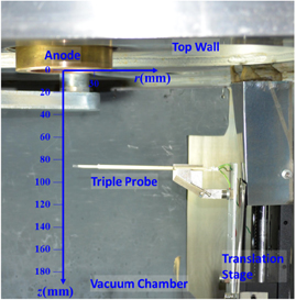
Figure 4. Construction of the triple probe and translation stages inside the vacuum chamber.
Download figure:
Standard image High-resolution imageDuring diagnosis, along the axial direction the initial point is z = 11 mm, and the spatial interval is 8 mm. Along the radial direction, the spatial interval is 4 mm, as shown in figure 5. At each axial position, the radial movement of the probe head is perpendicular to the probe, as illustrated in figure 5. To avoid damage from overheating, the probe is initially located at r = 120 mm. During sampling, the probe head moves at a speed of 10 mm s−1 into the diagnosis point, stops 2 s for sampling, then moves back to the initial position and waits 15 s for the next sampling, as shown in figure 5. The central point is first sampled. The resulting recording is shown in figure 6.

Figure 5. The temporal path line of the radial movement of the triple probe.
Download figure:
Standard image High-resolution image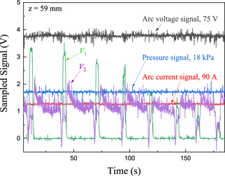
Figure 6. Typical sampled signals of the arc voltage, arc current, cathode chamber pressure, and V1 and V2 by the DAQ at an axial distance of 59 mm for the eight radial points under an arc current of 90 A.
Download figure:
Standard image High-resolution imageFigure 6 shows typical raw recording data of the experimental conditions of the arc voltage, arc current and cathode chamber pressure from the sensors, as well as the diagnosis signals U1 and U2 from the triple probe. It is located at z = 59 mm under an arc current of 90 A. The eight peaks of U2 correspond to the eight radial points from r = 0 mm to r = 28 mm. The top widths of the peaks are 2 s.
During data processing, all data are chosen with an almost steady arc voltage, a steady arc current and a steady cathode chamber pressure, and only the data in the time interval of 2 s are extracted. The stepped motors' power in the translation stage is still on during sampling, which interrupts the sensors and the probe and causes noise, as shown in figure 6. Thus, the data are first smoothed. However, fluctuations still exist in U1 and U2, as will be shown below.
3. Experiment results
The distribution patterns of ne and Te, obtained using equations (12) and (13), are shown in figures 7 and 8, respectively. Part of the data was previously published in [40]. Obviously, the patterns of ne resemble the propagation of waves downstream of the flow. The islets of relatively high ne correspond to the wave crests, such as in z = 35 mm–55 mm. As the arc current increases, the crests grow stronger, but the structure, i.e. the locations of the crests, remains unchanged.
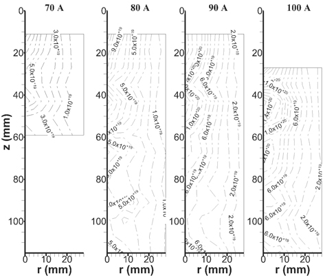
Figure 7. Distribution of the electron density at 70 A, 80 A, 90 A and 100 A. Part of the data was previously published [40].
Download figure:
Standard image High-resolution image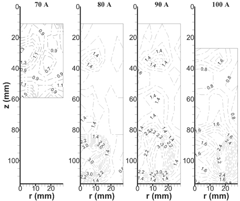
Figure 8. Distribution of electron temperature at 70 A, 80 A, 90 A and 100 A [40].
Download figure:
Standard image High-resolution imageThe Te patterns also demonstrate wave-like structures, but the wave crests deviate from the central axis. The deviation increases as the arc current increases. Similar to ne, the pattern structure remains unchanged. The absolute Te is apparently much higher downstream than upstream.
The axial distributions of ne at 80 A, 90 A and 100 A are shown in figure 9 (the upper part). The error bar of the data represents the temporal fluctuations during the sampling interval, as shown in figure 6. At 80 A, ne decreases significantly from z = 11 mm to 35 mm, corresponding to the expansion of the flow, increases abruptly from z = 35 mm to 43 mm, corresponding to compression, and then repeats the decreasing and increasing from z = 43 mm to 67 mm. At 90 A and 100 A, the behaviors of ne are almost the same as those of 80 A.
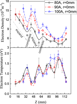
Figure 9. The axial distributions of the electron density (the upper) and the electron temperature (the bottom) along the central axis. The empty square points represent the results under arc current of 80 A, the empty circle points 90 A and the empty triangle points 100 A.
Download figure:
Standard image High-resolution imageThe axial distributions of Te at 80 A, 90 A and 100 A are shown in figure 9 (the bottom part). The values at z = 11 mm and z = 19 mm are 0.5–0.6 eV. The main tendency is that Te increases with the axial distance, but during expansion Te increases, and at the compression Te decreases.
Figures 10 and 11 show the radial distributions of ne and Te under an arc current of 90 A at axial positions of 11–67 mm. The maximum value of ne is 1.4 × 10²⁰ m−3 at the center of z = 11 mm, which decreases monotonically with the radial distance to 1.0 × 10¹⁹ m−3 at r = 28 mm.
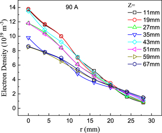
Figure 10. Radial distribution of ne at z = 11–67 mm under an arc current of 90 A.
Download figure:
Standard image High-resolution image
Figure 11. Radial distribution of Te at z = 11–67 mm under an arc current of 90 A.
Download figure:
Standard image High-resolution imageThe value of Te varies between 0.5–1.3 eV, while at the compression positions of z = 35 mm and 59 mm, Te varies between 1.0–1.9 eV. However, for all situations the radial distributions of Te are not monotonous, and the peaks always deviate from the center, as shown in figure 11.
4. Discussion
4.1. The wave structures in the jet
No shock structure was observed in the experiments. The wave patterns of ne and Te could be attributed to weak rarefaction waves. Our previous work showed that the velocity at the anode exit is approximately 1200 m s−1 [41], which corresponds to a translation energy of approximately 0.3 eV under the same typical discharge conditions and background pressure of 120 Pa. The translation energy is comparable to the gas kinetic energy, so the flow is compressible. Hence, it is possible that rarefaction waves exist in the flow.
Moreover, numerical simulations of the torch show that the local Mach number inside the anode is larger than 1, and that the pressure and density fluctuations of the flow are significant inside the anode, as shown in figures 12 and 13, respectively. The alternative expansion–compression structure would last in the jet. The simulations are based on the works of [42, 43], where specific information about the physical model, calculation mesh, etc, can be found. Since the model is based on the LTE assumption, which is questionable under this experimental condition, the simulation results only give a qualitative description of the plasma flow.
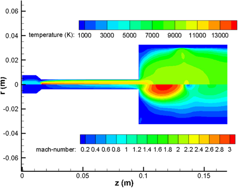
Figure 12. Numerical results of the temperature (the upper half) and the Mach number (the below half) inside the anode of the torch. The right side is the anode outlet.
Download figure:
Standard image High-resolution image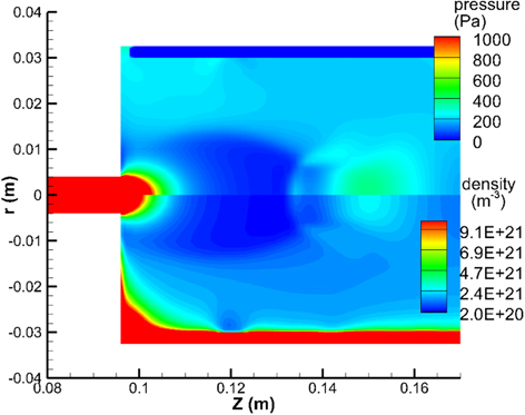
Figure 13. Numerical results of the pressure (the upper half) and the heavy-species density (the below half) inside the anode.
Download figure:
Standard image High-resolution imageThe compression or expansion of atoms leads to the same movements of ions due to effective collisions, and the electrons subsequently follow the movements due to the electric field caused by the compression or expansion of the ions. Therefore, the wave patterns shown in figures 7 and 8 are somewhat the projection of the flow waves.
4.2. Comparison of the ne and Te with the adiabatic case
4.2.1. The behaviour of ne
In the experimental works of [22–24], the main wave structure is a strong shock wave, but in our experiments the wave is an alternative expanding-compressing structure and rather weak. Comparing the experimental conditions, it was determined that both input powers are nearly equal, but the gas flow rate is much larger and the background pressure is higher in our experiments. According to the tendency of the shock location variation with the background pressure, as presented in [24, 27], the shock would move into the anode with a background pressure of 200 Pa. Due to the two abrupt expansions from the interelectrode to the anode and from the anode to the vacuum chamber, the plasma jet in this experiment is subjected to rarefication waves after exiting the anode.
Figure 14 shows the axial distribution of ne normalized by the value at z = 27 mm, which is the first common diagnosing position of the three arc currents, and the axis value is also normalized by d0 = 30 mm, which is the radius of anode. The data at z = 11–35 mm closely follow the curve of prediction 1 originating from equation (1). This means that the behavior in this spatial interval, corresponding to expansion (as shown in figure 9), is nearly adiabatic. The deduction of the curve of prediction 1 is illustrated briefly. According to equation (1),

Figure 14. Comparison between the experimental data of ne at arc currents of 80–100 A and the predictions of the scaling law of equation (1).
Download figure:
Standard image High-resolution imageCombined with equation (1) and eliminating n0,
which is the adiabatic curve of prediction 1. The data points of different arc currents in figure 14 become closer and even coincide, demonstrating that their behaviors are nearly governed by equation (15), despite the different characteristic values of n0 under each arc current.
At z = 35 mm, ne abruptly increases due to non-adiabatic compression and remains above adiabatic curve 1 in the later positions. After non-adiabatic compression, the behavior of the electron is again nearly adiabatic, and this phenomenon happens again after non-adiabatic compression at z = 59 mm, as illustrated by adiabatic prediction curves 2 and 3 in figure 14. The deduction of those two curves has the same process, unless using the reference ne values at z = 43 mm and 67 mm, respectively.
and
Equations (16) and (17) are the adiabatic curves of prediction 2 and prediction 3, respectively, with density transformations on the right-hand sides because all the ne values in figure 14 are normalized by ne (z = 27 mm).
Curve 1–3 are similar because of the adiabatic characteristics, but correspond to different values of n0, even for the same arc current conditions. The larger value of n0 at a constant arc power corresponds to a higher ionization rate of the plasma jet. Each non-adiabatic compression increases the value of n0, indicating that significant ionization occurs. This deduction could be confirmed from the experiments. The radial distribution tail of ne at z = 43 mm almost coincides with z = 35 mm, while the other part of the distribution is significantly larger, as shown in figure 10. The larger part at z = 35 mm is far more than that caused by the flow compression. In addition, the values of Te at z = 35 mm and 59 mm are much larger than those at nearby positions, which increases the ionization rate, as shown in figure 9. Moreover, Curves 1–3 are gradually closer, and the non-adiabatic compressions become weaker, demonstrating a decreasing strength in the ionization.
4.2.2. The effect of metastable atoms
The physics behind these phenomena is the process associated with ionization. The ionization rate, named R, is
where n is the density of the atom species to be ionized, v0 is the collisional velocity corresponding to the ionization energy. The ionization of argon atom from ground state requires an energy of 15.76 eV, while ionization from the metastable state requires about 4.11 eV. Thus, the presence of metastable atoms provides a large possibility for the ionizations in each compression regions. Since the ionization rate is linearly related to the density, the metastable density is a critical parameter. Metastable atoms are mainly produced by electron collisions with radiative lifetimes of about 1.3 to 55.9 s (see table 2.3 in [44]), which is much larger than the drift time of the plasma plume, but it may also be quenched by electron collision. An estimate of the density of metastable atoms will help to gain insight into the non-adiabatic phenomena. In the following part, an approximate calculation of the metastable atoms is implemented based on a simple collision model and reaction rates.
The main electron collision reactions and rate coefficients [35, 45, 46] in a partially ionized argon plasma are listed in table 1 and plotted in figure 15. The units of Te and ne are eV and m−3, respectively. The rate coefficients are in the form of interpolations of the integrals in equation (18) based on collisional cross-section data. In literatures, reaction 6 in table 1 produces excited atom, i.e. Ar(4s), which includes two metastable levels (1s5 and 1s3) and two resonance levels (1s4 and 1s2). Resonance levels are usually excited by resonance transitions with a lifetime of a few nanoseconds [47], which are not considered here. Omitting the resonance levels would lead to an overestimation of Qgm and Qtri by a factor of about 2 times if the level group of the reaction is homogeneous. However, this does not cause a large error because Qgm and Qtri are rather small in the Te range of interest and the rate of reaction 6 is proportional to ne 3, moreover, Te which is mainly influenced by reactions 3 and 6 is obtained by diagnostics.
Table 1. Electron collisional reactions and the rate coefficients.
| No. | Reaction | Rate coefficient |
|---|---|---|
| 1 | e + Arm → 2e + Ar+ | Qmi = 2.0 × 10⁻¹³ exp(−6.2/Te) (m3 s−1) |
| 2 | e + Arm → e + Ar | Qmg = 4.8 × 10⁻¹⁶ Te 0.5 (m3 s−1) |
| 3 | e + Ar → e + Arm | Qgm = 4.9 × 10⁻¹⁵ Te 0.5 exp(−11.65/Te) (m3 s−1) |
| 4 | e + Ar → 2e + Ar+ | Qgi = 1.27 × 10⁻¹⁴ Te 0.5 exp(−15.76/Te) (m3 s−1) |
| 5 | e + Ar+ → Ar + hν | Qig = 2.01 × 10⁻¹⁹ Te −0.5 (m3 s−1) |
| 6 | 2e + Ar+ → e + Arm | Qtri = 2.0 × 10−39 Te −4.5 ne (m3 s−1) |

Figure 15. Rate coefficients of electron-impact reactions as a function of electron temperature.
Download figure:
Standard image High-resolution imageConsider a plasma system consisting of electrons, ions, metastable atoms and ground state atoms, where the electrons and ions have the same density, i.e. ne, and all the component has the same velocity,  . The law of mass conservation of the electrons is

which could be transformed into
Similarly, the laws of mass conservation for metastable atoms and total species are

where nt = ni + nm + ng = ne + nm + ng. Combining equa-tions (20)–(22),

where  for j = e, m. In the plasma plume, ξe ≪ 1, ξm ≪ 1. Hence, a differential relation between ξm and ξe could be obtained by dividing equation (24) by (23)

The spatial distribution of the metastable density ratio ξm along the central axis is calculated by implicit discretization of equation (25), while the diagnostic results of electron density and electron temperature are used to calculate the rate coefficients. The integration of equation (25) requires an initial value, but which is unknown, so in the calculation, the ξm at initial point (i.e. Z = 11 mm, denoted ξm,11 mm) is tested over a wide range with 16 values of 0.0001, 0.001, 0.002, 0.003, 0.004, 0.005, 0.006, 0.007, 0.008, 0.009, 0.01, 0.02, 0.03, 0.04, 0.05 and 0.1. nt is set to 1022 m−3, corresponding to the characteristic gas temperature of 1450 K [48].
Figures 16 and 17 show the calculated axial distributions of metastable atoms under arc currents of 80 A and 90 A, respectively. In the case of 80 A, the axial density distributions with ξm,11 mm ⩽ 0.01 converge rapidly into a curve, as shown in figure 16. This means that metastable atoms along the axial direction are mainly produced by local electron-impact collisions, as in reactions 1–3 and 6 in table 1. However, as ξm,11 mm increases, the initial metastable density has a strong influence on the reaction within the downstream plume, and leads to negative values of ξm, which are non-physical. The main reason is that the initial values deviate far from the true value, leading numerical oscillations. In the case of 90 A, the distributions also converge into a curve, but oscillations and negative values of ξm,11 mm occur as ξm,11 mm > 0.01 or 0.000 1 < ξm,11 mm < 0.008, as shown in figure 17.

Figure 16. Calculated axial distributions of the metastable density ratio using different initial ratios at Z = 11 mm, in which the diagnostic results of arc currents of 80 A are used.
Download figure:
Standard image High-resolution image
Figure 17. Calculated axial distributions of the metastable density ratio using different initial ratios at Z = 11 mm, in which the diagnostic results of arc currents of 90 A are used.
Download figure:
Standard image High-resolution imageDue to the independence on ξm,11 mm, the two converged curves in figures 16 and 17 should be the density distributions of metastable atoms. In the downstream expansion regions, the metastable density ratio is 0.001–0.004 for 80 A, and is 0.002–0.007 for 90 A, wherefore the metastable density increases with input power of the plasma.
Comparing with figure 9, it is found that the density of metastable atoms increases in the expansion region and decreases in the compression region. Thus, the presence of metastable atoms is an important reason for ionization in the weakly compressible plasma jet. The calculations show that the metastable atoms are mainly produced locally as a result of competition for the reactions 1–6 listed in table 1. Thus, the metastable atoms act as effective energy exchange channels between electrons and heavy particles.
The experimental data in figure 14 almost agree with the prediction of the curves, but are not as good as the prediction in [24, 27] where the plasma jet experienced strong expansion. The main reason is that each species in the plasma flow is not absolutely adiabatic, and energy transfer processing, such as ionization and recombination, is lasting along the flow. Another reason is the error in the probe diagnosis. Ion saturation current variation [28] and the influence of the alignment [20] would be the source of errors. The ion saturation current could increase about 20% as the biased voltage of the probe increase to 35 V in the plasma with electron density of about 1020 m−3 as observed in a recent experiments. In our experiments, the floating pin 3 is right behind the pin 2, causing a shadowing effect. This effect could lead negative measurement error in Te of about 50% in downstream and in ne of about 29%–37% in the whole plume. In addition to the ion saturation current variation and the influence of the alignment, the thermal emission of the probe could be a significant effect, which will be further studied.
4.2.3. The behaviour of Te
The axial distribution of Te apparently does not agree with the scaling law of equation (2), since it predicts a monotonously increasing trend; however, this is obviously not in this experiment. The phenomenon that radial-distribution peaks deviated from the central axis also appeared in other experimental works with different diagnosis methods [24, 49]. Two physical processes simultaneously result in this phenomenon. The first reason is that electron collision ionizations cost the electrons kinetic energy, especially the high-rate ionizations of metastable atoms, as shown in figure 15, which make Te decrease dramatically in the central region.
Another reason is the existence of an electric field aroused by the ambipolar diffusion, to which the electrons are sensitive. In a plasma without a net current, the electric field is related to Te, the gradient of ne [50],

where D is the diffusion coefficient and μ is mobility, and the subscripts i and e denote ions and electrons, respectively. According to equation (26), the electric field strength and the streamline of the field are calculated using the diagnosis values of Te and ne, as shown in figure 18. The field strength is relatively weak around the central area, and the field direction is almost radial. The electric field mainly heats the electrons due to the large mass ratio of mi/me and much faster energy relaxation [51, 52]. Subsequently, the electron temperature is higher in the region of the stronger electric field. The energy contained in the electric field originates from the internal energy of the electron gas around the center. This is because the electrons have much greater mobility and build up the electric field through the density gradient, as described in (26), which dissipates the internal energy gradient of the electrons. Therefore, the radial peak deviation of Te from the center is partly attributed to the radial energy transport and dissipation of the electrons.
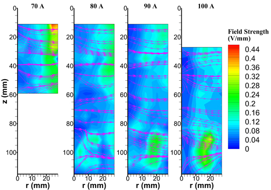
Figure 18. The electric field strength and the streamline of the field calculated from the experimental data with arc currents of 70–100 A.
Download figure:
Standard image High-resolution image4.3. Dependence of ne and Te on the input power
As shown in figures 7 and 9, the increase of the arc current results in a monotonic increase in ne. However, the behavior of Te is much different. Figure 19 shows the variations in Te with arc currents of 70–100 A at axial distances of z = 27–59 mm and radial distances of r = 0–28 mm. It is clearly shown that at r = 0–8 mm, Te decreases with the arc current, and the decrease is monotonous only for z = 27 mm and z = 51 mm, while in other positions, Te decreases and increases at certain arc currents.
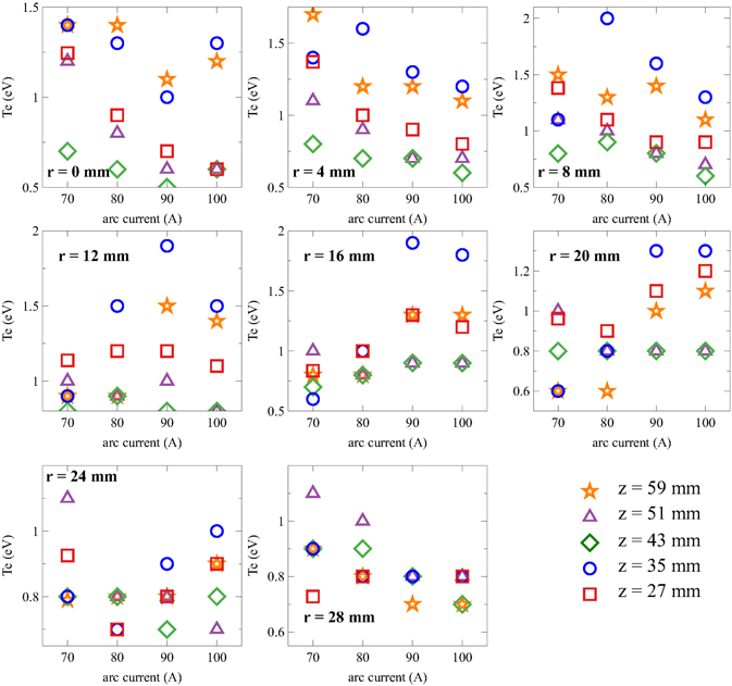
Figure 19. Variations in Te with arc currents at r = 0–28 mm and z = 27–59 mm.
Download figure:
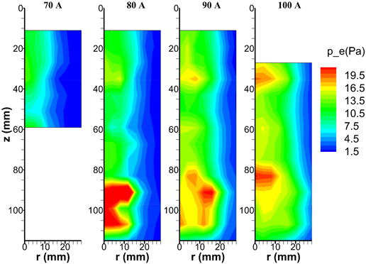
Standard image High-resolution imageThe phenomenon where Te decreases with the input power has seldom been reported. Te should increase with the input power inside the arc channel where the thermodynamic state is close to LTE. However, the processes of expansion–compression and ionization-recombination redistribute the energy of the plasma jet among different energy types, i.e. translation energy, kinetic energy, internal energy, entropy, etc, and different spatial positions, resulting in the plasma deviating from the initial state. Despite these complicated processes, the total kinetic energy flux of the electrons increases with the input powers, since
According to the diagnosis results, the electron pressure increases with the arc current, as shown in figure 20. Hence, δEkinetic/δI > 0, which is reasonable.
Figure 20. The pressure of the electrons calculated using the experimental data.
Download figure:
Standard image High-resolution image
5. Conclusion
In this paper, a high-speed plasma jet was diagnosed using an electrostatic triple probe, which is produced by a DC plasma torch with an abruptly expanding anode. The results of two-dimensional patterns of ne and Te with 70–100 A were presented containing 80 spatial points.
First, the wave structure in the patterns was discussed and analysed as the projection of the flow waves and was compared with previous studies of strong compressible plasma flows. The repeating expansions of ne are nearly adiabatic, but the compressions are non-adiabatic and make ne increase significantly. The main reason for the non-adiabatic behavior is analysed based on a simple electron collision model, in which the metastable density is calculated. It is found related to the collisional ionizations of metastable atoms, which occur in the entire flow, but become stronger at each compression.
Second, the peaks of the radial distribution of Te deviate from the central point. This was explained as resulting from the electron collisional ionizations in the central area, and the radial energy transport and dissipation of the electrons from the center into the peripheral position.
Last, it was observed that Te decreases with input power at some positions. This could be the result of multi-physics processes of expansion–compression and ionization-recombination. However, the total kinetic energy flux of electrons still increases with the input power.
Acknowledgments
This work was supported by the Strategic Priority Research Program of the Chinese Academy of Sciences (Grant No. XDA17030100), the National Natural Science Foundations of China under Grant 11735004 and Grant 11575273, and the Hainan Province Science and Technology Special Fund (Grant No. ZDKJ2019004). Jinwen Cao was partially supported by the LHD Youth Innovation Fund from the State Key Laboratory of High Temperature Gas Dynamics.
Data availability statement
The data that support the findings of this study are available upon reasonable request from the authors.