
Abstract
Objective. The aim of the study is to investigate the effect of the signal sampling frequency and low-pass filtering on the accuracy of the localisation of the fiducial points of the photoplethysmographic signal (PPG), and thus on the estimation of the blood pressure (i.e. the accuracy of the estimation). Approach. Statistical analysis was performed on 3,799 data samples taken from a publicly available database. Four PPG fiducial points of each sample signal were examined in the study. Main results. Simulation suggests that for noise-free data, cubic spline interpolation causes the sampling frequency (in the considered range of 62.5–500 Hz) to have only limited influence on localisation of the fiducial point. Better results were obtained for the pulse transit time (PTT) than pulse arrival time (PAT) approach. The acceptable filter band depends on the selected fiducial point and PAT or PTT approach. The best results were obtained for the tangent fiducial point. Significance. The presented results make it possible to estimate the minimum requirements for the sampling frequency and filtering of the PPG signal in order to obtain a reliable estimation of blood pressure.
Export citation and abstract BibTeX RIS

Content from this work may be used under the terms of the Creative Commons Attribution 4.0 licence. Any further distribution of this work must maintain attribution to the author(s) and the title of the work, journal citation and DOI.
1. Introduction
Blood pressure (BP) monitoring can be used to assess state of the circulatory system, in particular to detect dangerous episodes of hypertension or hypotension (Mendis et al 2011, Lackland and Weber 2015). Thus, non-invasive and continuous BP monitoring, especially in the elderly, is both an important and challenging issue. However, there are only a few measurement techniques that can achieve this goal. The problem is more challenging when restricted only to wearable devices. Taking the associated limitations into account, the dependence of pulse wave velocity (PWV) on BP is commonly considered a possible phenomenon to utilise. PPG, sometimes in conjunction with other techniques, is used for its determination in most cases described in the literature. Going into the details, there are two different techniques based on this approach. The first is based on calculating the PWV, assuming that the distance from a heart to the PPG measurement point on a distal artery is known. As a result, the pulse pressure propagation time between the heart and the measurement point is determined as the time difference between the occurrence of the R wave in the ECG and the arrival time of the pulse pressure wave at the location of the PPG sensor. This method is known as pulse arrival time (PAT). The other approach is based on the simultaneous measurement of two PPG signals at distant points, which are preferably located on a selected artery. This approach is known as the pulse transit time (PTT) method. The disadvantage of the PAT-based approach is the influence of the pre-ejection period (PEP) on the measurement results (PAT = PEP+PTT). Monitoring BP with an accuracy of a few mmHg is equivalent to achieving a resolution of PTT or PAT determination equal to a single millisecond (Proença et al 2010, Poliński et al 2019). Therefore, it is a very important to set the appropriate parameters of the measurement system to meet such requirements.
Wearable devices, as applied for health monitoring, is a rapidly developing area of research. Nevertheless, in spite of spectacular achievements, they are often shaped by general requirements, e.g. the ability to perform long-term monitoring. As a result, they are being optimised to reduce power consumption. This is achieved, among others, by reducing the sampling rate of the measured signals (see, for example (Polimeni et al 2014, Gircys et al 2019, Mousavi et al 2019, Yoon et al 2009, He et al 2022, McCombie et al 2006), where the sampling frequency varies from 30 Hz up to 20 kHz). Moreover, to reduce the noise in such systems, the signals are low-pass filtered using filters of different cut-off frequencies (see, for example (Zhang and Feng 2017, He et al 2022, Agrò et al 2014, McCombie et al 2006), where the cut-off frequency varies from 5 Hz to 25 Hz). It is typically assumed that the bandwidth of the PPG signal is small. This explains the strong filtering of the signal and the relatively low sampling frequency. However, considering the measurement resolution requirements imposed by the blood pressure estimation accuracy, the requirements can be increased. This is the reason for the analyses performed in this paper.
The PPG sampling frequency and cut-off frequency of the low-pass filter determine the shape of the PPG signal. The features of the PPG waveform, as measured at a low sampling rate, were investigated in (Fujita and Suzuki 2019). However, this study did not include the fiducial point's localisation problem. The examined sampling frequency span was relatively large (240 Hz original, downsampled to 120, 60, 30, 20 and 10 Hz), but the signal was heavily filtered in all considered cases (low-pass filter with cut-off frequency 10 Hz). The features of the PPG signal were analysed in (Polimeni et al 2014), however, the signal was only sampled at one frequency equal to 120 Hz. The cubic spline and parabola interpolation of a subsampled signal for accurate heart rate variability analysis was examined in (Béres and Hejjel 2021). In the paper (Liu et al 2021), the effect of the PPG signal morphology and type of pulse feature on the filtering-induced time shift were investigated. There are other papers which are connected to the analysed problem. For example, the optimal fiducial points of the PPG signal for pulse rate variability analysis were considered in (Peralta et al 2019) and selection of the minimal and acceptable sampling frequency of the PPG signal when monitoring a pulse rate by means of mobile and wearable technology was examined in (Béres et al 2019). The performance of different PWV algorithms was assessing in (Gaddum et al 2013). However, the simultaneous influence of the considered parameters on the accuracy of localisation of the PPG fiducial points were not been examined in any of the above-mentioned studies. In many studies presenting the results of blood pressure estimates by means of PTT or PAT measurements, the accuracy and resolution of localisation of fiducial PPG points is of the same order as their changes involved by blood pressure variability being estimated. This resolution is limited, inter alia, by the sampling frequency of the PPG signal, measurement noise and the procedures used in its removal (e.g. by low-pass filtering).
The study shown in this paper can be used not only for an indirect assessment of the blood pressure, i.e. based on PAT or PTT. This is because the signal pre-processing procedures that could be included in this category (e.g. low-pass filtering to remove noise) are also used in many other applications, including machine learning. The aim of the work is therefore to examine the influence of the signal sampling frequency and low-pass filtering on the accuracy of localising fiducial PPG points, and thus on the accuracy of estimating the blood pressure, assuming fixed conditions of examination by utilising a 'clear' and stationary PPG signal.
2. Material and methods
A basic set of the analysed signals, the synthetic ones, was obtained from (Charlton et al 2019). More details about the model are given in (Charlton et al 2019). The analysis was conducted for PPG waves sampled at 500 Hz. Only data for physiologically plausible virtual subjects (3,837 cases) were considered. However, an additional 38 PPG signals were excluded from the analysis due to their atypical form (see figure 1). Thus, only 3,799 cases were further analysed. These signals were considered as reference ones and were used for creating sets of signals characterised by different sampling rates and frequency spectrums. To test the influence of the signal sampling rate on the fiducial point's localisation accuracy, the original signals were re-sampled at frequencies of 250, 125, 100 and 62.5 Hz. This was done by taking every 2nd, 4th, 5th and 8th sample from the original signal. This procedure multiplied the number of signals of lower sampling rates, respectively, 2, 4, 5 and 8 times, relative to the initial sample from which signals with a lower sampling rate were selected. It should be underlined that these signals differed in phase between each other. Then, each signal was filtered by means of a low-pass filter as in (Poliński et al 2021), assuming that the Nyquist criterion was met. All filters were designed in Matlab using filterDesigner. The FIR filters with fpass equal to 10, 15, 20, 30 and 60 Hz and fstop 10 Hz higher than fpass were used. The Apass was equal to 1 dB, while Astop was equal to 80 dB. The Kaiser window was used. The filter order was equal to 251, 126, 63, 51 and 32 for sampling frequencies equal to 500 Hz, 250 Hz, 125 Hz and 62.5 Hz, respectively. The signals were filtered forwards and backwards to remove the phase shift inherent in digital filters. To perform the filtering and to avoid the influence of the phenomenon of transitional states on the results, each signal was lengthened in time by its repetition as many times as was needed. Since the measurement signal can be first filtered and then re-sampled, this sequence of operations was also analysed (first filtering the signal with a sampling frequency 500 Hz using filters with a cut-off frequency of 10 Hz, 15 Hz, 20 Hz, 30 Hz and 62.5 Hz, and then re-sampling, as described above).
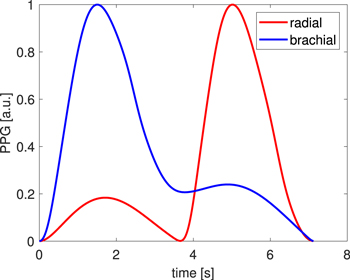
Figure 1. Example of excluded data.
Download figure:
Standard image High-resolution imageIn general, the PPG signal is modified as it propagates along the vessel and also when it is processed by a measurement system. Thus, the selection of the measurement location in the circulatory system has a crucial influence on the result of the analysis performed. It was decided that recordings from selected points of the brachial and radial arteries would be the subject of this analysis, as this is the most common approach presented in the literature. For each of the PPG signals and for each of the chosen arteries, four fiducial points were determined. The first (marked by a square in figure 2) was the signal minimum, the second (marked by a triangle in figure 2) was the signal maximum, the third (marked by an asterisk in figure 2) was the maximum of the signal's first derivative (a forward quotient was used to estimate the derivative), and the fourth (marked by a circle in figure 2) was the point determined by the cross-section of two lines, one being tangent to the minimal value of the signal, while the other was tangent to the signal at its maximal slope (maximal value of the first derivative). In the last case, the tangent was calculated based on five points near the maximal slope using the least squares approach (Mukkamala et al 2015, Poliński et al 2021). An example of the locations of the fiducial points of the PPG signal is presented in figure 2. Due to the visibility of the signal together with its derivative, the Y axis is in arbitrary units. Before estimating the location of the fiducial points, the analysed signal was interpolated using cubic spline interpolation (the spline Matlab function was used) like in (Charlton et al 2017). This was done in order to improve the accuracy of the location of the fiducial points, especially for lower sampling rates. After interpolation, the accuracy of the location of the fiducial points was increased to a resolution of 0.002 ms (except for the tangent point, for which there was a higher resolution). Due to the variety of shapes of the PPG signal, determination of the location of the fiducial points was limited to approximately the range −64 ms before the minimum of the original (not interpolated) PPG signal and +64 ms after the maximum of the original (not interpolated) PPG signal. For a sampling frequency equal to 100 Hz, it was ±70 ms. All fiducial points were determined using a procedure developed in Matlab.
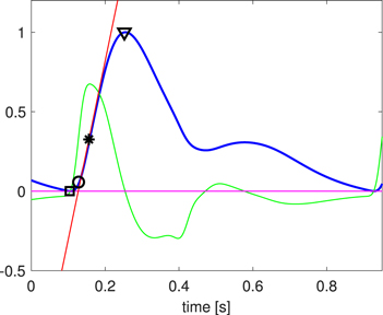
Figure 2. Fiducial point localisation (black markers) on signal (blue) and first derivative of signal (green).
Download figure:
Standard image High-resolution imageThe errors of the fiducial point localisations were calculated as absolute values of the difference between the localisation of the fiducial point for a chosen signal (re-sampled and/or low-pass filtered, after its interpolation) and the reference signal. The point localisations, as determined from the original signals (without any filtering), sampled with fs = 500 Hz and then interpolated to 500 kHz, were taken as the reference.
The following error measures were determined: mean error and standard deviation of errors for each fiducial point and for each modified signal (re-sampled and/or filtered). These measures were used to estimate the accuracy (in milliseconds) of the determination of the fiducial points. In turn, they could illustrate the accuracy of the BP determination according to error propagation theory, as the BP, in the approach discussed in the paper, is calculated as a function of the pulse wave velocity. The analysis of the influence of noise on the results was not included in the paper. The reasons for this decision are presented in the Discussion section.
3. Results
Processing signals changes their shape, e.g., in response to the low-pass filtering applied. However, the range and form of the changes depend on the relation between their spectrum and the filter's parameters (figure 3). This is also noticeable when localisation of the tangent point is considered (figure 4, where the influence of low-pass filtering on its localisation was examined).
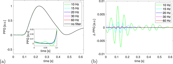
Figure 3. (a) The signals' shapes change due to low-pass filtering (fs = 500 Hz) and (b) Difference (Δ PPG) between filtered and unfiltered (reference) signals.
Download figure:
Standard image High-resolution image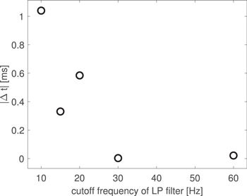
Figure 4. Example of the influence of low-pass filter cut-off frequency (x-axis) on localisation of tangent point (time difference between tangential points determined for a non-processed and filtered signals).
Download figure:
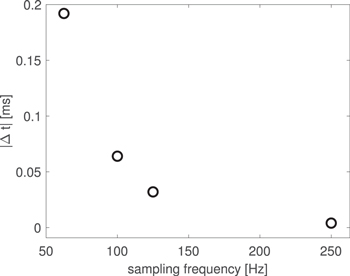
Standard image High-resolution imageA similar scatter of the PPG's signal minimum position was noticeable in response to different sampling rates (figure 5).
Figure 5. Influence of the sampling frequency on the signal minimum localisation. Time difference between position of the minimum of the signals sampled at frequency equal to 62.5, 100, 125 and 250 Hz with respect to the reference one, i.e. sampled at 500 Hz.
Download figure:
Standard image High-resolution image
All values for the mean errors and the standard deviations (std) presented in the tables are given in milliseconds. The analysed fiducial points described in the tables as min, max, diff and tg, correspond to the minimum, maximum, maximum of the first derivative, and intersection point of the two tangent lines. The results are presented for the PPG signals, for the fiducial point localisation on a single artery (PAT approach) and for the difference between the fiducial points localisations on the radial and brachial arteries (PTT approach).
The errors, i.e. (mean ± std), introduced by filtering the original signal measured on the radial artery and characterised by different cut-off frequencies are summarised in table 1. Please note that the values 0.00 in the tables do not mean no error. They mean that the error is less than 0.005 ms.
Table 1. Filter bandwidth effect for interpolated PPG (radial artery, fs = 500 Hz). Labels in the table: min, max, diff, and tg, correspond to minimum, maximum, maximum of the first derivative, and intersection point of the two tangent lines.
| Filter [Hz] | min | max | diff | tg |
|---|---|---|---|---|
| 60 | 0.00 ± 0.01 | 0.00 ± 0.01 | 0.02 ± 0.04 | 0.00 ± 0.00 |
| 30 | 0.13 ± 0.15 | 0.06 ± 0.17 | 0.60 ± 0.62 | 0.03 ± 0.03 |
| 20 | 0.69 ± 0.60 | 0.27 ± 0.54 | 3.13 ± 2.71 | 0.19 ± 0.14 |
| 15 | 1.76 ± 1.15 | 0.45 ± 1.20 | 3.04 ± 2.30 | 0.53 ± 0.24 |
| 10 | 4.58 ± 1.39 | 0.82 ± 2.66 | 4.41 ± 2.53 | 1.27 ± 0.39 |
The errors (mean ± std) for the difference in the localisation of the fiducial points on the radial and brachial arteries for the original signal are presented in table 2.
Table 2. Filter bandwidth effect for interpolated PPG on the time difference as determined between fiducial points on the radial and brachial arteries, fs = 500 Hz. Labels in the table: min, max, diff, and tg, correspond to minimum, maximum, maximum of the first derivative, and intersection point of the two tangent lines.
| Filter [Hz] | min | max | diff | tg |
|---|---|---|---|---|
| 60 | 0.01 ± 0.02 | 0.01 ± 0.04 | 0.08 ± 0.29 | 0.00 ± 0.01 |
| 30 | 0.23 ± 0.11 | 0.11 ± 0.35 | 0.80 ± 1.21 | 0.04 ± 0.04 |
| 20 | 0.65 ± 0.36 | 0.35 ± 1.33 | 2.67 ± 3.11 | 0.19 ± 0.15 |
| 15 | 0.85 ± 0.76 | 0.49 ± 1.65 | 2.73 ± 2.56 | 0.20 ± 0.18 |
| 10 | 0.88 ± 0.64 | 0.92 ± 3.11 | 2.70 ± 2.60 | 0.27 ± 0.20 |
For lower sampling frequencies (62.5 Hz–250 Hz), the mean errors and their standard deviations are listed in the form of value ranges (symbol '–' in the tables). This is due to the different starting points, which can be used to verify the influence of the initial phase of the signal on the estimation results. The results in table 3 are provided for a brachial artery signal sampled at a frequency equal to 250 Hz. Next, the effect of the sample filtration on determining the time difference between the localisation of the fiducial points on the radial and brachial arteries are presented in table 4.
Table 3. Filter bandwidth effect for interpolated PPG (brachial artery, fs = 250 Hz). Labels in the table: min, max, diff, and tg, correspond to minimum, maximum, maximum of the first derivative, and intersection point of the two tangent lines. n.f. means not filtered. The point localisations, as determined from the original signals, sampled with fs = 500 Hz and then interpolated to 500 kHz, were taken as the reference.
| Filter [Hz] | min | max | diff | tg |
|---|---|---|---|---|
| n.f. | 0.00–0.01 | 0.00–0.00 | 0.04–0.05 | 0.00–0.00 |
| ±0.00–0.01 | ±0.00–0.00 | ±0.05–0.31 | ±0.00–0.00 | |
| 60 | 0.01–0.02 | 0.01–0.01 | 0.10–0.11 | 0.00–0.00 |
| ±0.03–0.03 | ±0.04–0.04 | ±0.29–0.31 | ±0.01–0.01 | |
| 30 | 0.30–0.30 | 0.10–0.10 | 0.70–0.70 | 0.04–0.04 |
| ±0.26–0.26 | ±0.33–0.33 | ±1.17–1.18 | ±0.04–0.04 | |
| 20 | 1.10–1.10 | 0.33–0.33 | 3.96–3.96 | 0.21–0.21 |
| ±0.64–0.64 | ±1.26–1.26 | ±3.67–3.67 | ±0.18–0.18 | |
| 15 | 2.39–2.39 | 0.50–0.50 | 4.51–4.51 | 0.47–0.47 |
| ±1.02–1.02 | ±1.16–1.16 | ±3.46–3.46 | ±0.33–0.33 | |
| 10 | 5.40–5.40 | 0.91–0.91 | 4.23–4.23 | 1.50–1.50 |
| ±1.35–1.35 | ±1.79–1.79 | ±2.59–2.59 | ±0.48–0.48 |
Table 4. Filter bandwidth effect for interpolated PPG on the time difference as determined between fiducial points on the radial and brachial arteries, fs = 250 Hz. Labels in the table: min, max, diff, and tg, correspond to minimum, maximum, maximum of the first derivative, and intersection point of the two tangent lines. n.f. means not filtered. The point localisations, as determined from the original signals, sampled with fs = 500 Hz and then interpolated to 500 kHz, were taken as the reference.
| Filter [Hz] | min | max | diff | tg |
|---|---|---|---|---|
| n.f. | 0.00–0.01 | 0.00–0.00 | 0.06–0.07 | 0.00–0.00 |
| ±0.00–0.01 | ±0.00–0.00 | ±0.06–0.31 | ±0.00–0.00 | |
| 60 | 0.01–0.01 | 0.01–0.01 | 0.11–0.12 | 0.00–0.00 |
| ±0.02–0.03 | ±0.04–0.04 | ±0.28–0.30 | ±0.01–0.01 | |
| 30 | 0.23–0.23 | 0.11–0.11 | 0.80–0.80 | 0.04–0.04 |
| ±0.11–0.11 | ±0.35–0.35 | ±1.21–1.21 | ±0.04–0.04 | |
| 20 | 0.65–0.65 | 0.35–0.35 | 2.67–2.67 | 0.19–0.19 |
| ±0.35–0.36 | ±1.33–1.33 | ±3.11–3.12 | ±0.15–0.15 | |
| 15 | 0.85–0.85 | 0.49–0.49 | 2.73–2.74 | 0.20–0.20 |
| ±0.76–0.76 | ±1.66–1.66 | ±2.56–2.57 | ±0.18–0.18 | |
| 10 | 0.88–0.88 | 0.92–0.92 | 2.70–2.70 | 0.27–0.27 |
| ±0.64–0.64 | ±3.12–3.12 | ±2.60–2.60 | ±0.20–0.20 |
The results of filtering effect for radial artery signal sampled at 125 Hz frequency are presented in table 5.
Table 5. Filter bandwidth effect for interpolated PPG (radial artery, fs = 125 Hz). Labels in the table: min, max, diff, and tg, correspond to minimum, maximum, maximum of the first derivative, and intersection point of the two tangent lines. n.f. means not filtered. The point localisations, as determined from the original signals, sampled with fs = 500 Hz and then interpolated to 500 kHz, were taken as the reference.
| Filter [Hz] | min | max | diff | tg |
|---|---|---|---|---|
| n.f. | 0.00–0.01 | 0.00–0.00 | 0.06–0.07 | 0.00–0.00 |
| ±0.00–0.01 | ±0.00–0.00 | ±0.06–0.31 | ±0.00–0.00 | |
| 30 | 0.13–0.14 | 0.06–0.06 | 0.63–0.65 | 0.03–0.03 |
| ±0.15–0.16 | ±0.16–0.17 | ±0.62–0.66 | ±0.02–0.03 | |
| 20 | 0.69–0.70 | 0.27–0.27 | 3.12–3.14 | 0.19–0.20 |
| ±0.60–0.60 | ±0.54–0.55 | ±2.70–2.72 | ±0.14–0.14 | |
| 15 | 1.76–1.76 | 0.45–0.45 | 3.04–3.05 | 0.53–0.53 |
| ±1.15–1.15 | ±1.19–1.20 | ±2.30–2.31 | ±0.24–0.24 | |
| 10 | 4.57–4.57 | 0.82–0.82 | 4.41–4.41 | 1.27–1.27 |
| ±1.39–1.39 | ±2.66–2.67 | ±2.53–2.53 | ±0.39–0.39 |
The results of the time delay between the PPG signals measured on the radial and brachial arteries sampled at a frequency equal to 100 Hz are presented in table 6.
Table 6. Filter bandwidth effect for interpolated PPG on the time difference as determined between fiducial points on the radial and brachial arteries, fs = 100 Hz. Labels in the table: min, max, diff, and tg, correspond to minimum, maximum, maximum of the first derivative, and intersection point of the two tangent lines. n.f. means not filtered. The point localisations, as determined from the original signals, sampled with fs = 500 Hz and then interpolated to 500 kHz, were taken as the reference.
| Filter [Hz] | min | max | diff | tg |
|---|---|---|---|---|
| n.f. | 0.00–0.01 | 0.00–0.00 | 0.06–0.07 | 0.00–0.00 |
| ±0.00–0.01 | ±0.00–0.00 | ±0.06–0.31 | ±0.00–0.00 | |
| 30 | 0.19–0.31 | 0.10–0.11 | 0.83–0.95 | 0.04–0.04 |
| ±0.11–0.12 | ±0.33–0.34 | ±1.11–1.43 | ±0.04–0.04 | |
| 20 | 0.62–0.68 | 0.34–0.35 | 2.68–2.82 | 0.19–0.19 |
| ±0.34–0.37 | ±0.89–1.34 | ±3.04–3.17 | ±0.15–0.15 | |
| 15 | 0.84–0.86 | 0.49–0.49 | 2.71–2.80 | 0.20–0.21 |
| ±0.75–0.76 | ±1.66–1.66 | ±2.55–2.59 | ±0.18–0.18 | |
| 10 | 0.88–0.89 | 0.95–0.97 | 2.67–2.73 | 0.27–0.27 |
| ±0.64–0.64 | ±3.33–3.61 | ±2.59–2.62 | ±0.20–0.20 |
The results for a radial artery signal sampled at 62.5 Hz are presented in table 7, and the time delays between signals measured on the radial and brachial arteries and sampled at the same frequency are gathered in table 8.
Table 7. Filter bandwidth effect for interpolated PPG (radial artery, fs = 62.5 Hz). Labels in the table: min, max, diff, and tg, correspond to minimum, maximum, maximum of the first derivative, and intersection point of the two tangent lines. n.f. means not filtered. The point localisations, as determined from the original signals, sampled with fs = 500 Hz and then interpolated to 500 kHz, were taken as the reference.
| Filter [Hz] | min | max | diff | tg |
|---|---|---|---|---|
| n.f. | 0.00–0.01 | 0.00–0.00 | 0.06–0.07 | 0.00–0.00 |
| ±0.00–0.01 | ±0.00–0.00 | ±0.06–0.31 | ±0.00–0.00 | |
| 20 | 0.74–0.89 | 0.24–0.25 | 3.02–3.37 | 0.20–0.22 |
| ±0.60–0.73 | ±0.51–0.52 | ±2.78–3.02 | ±0.14–0.16 | |
| 15 | 1.78–1.85 | 0.43–0.45 | 3.03–3.17 | 0.54–0.56 |
| ±1.14–1.18 | ±0.63–1.20 | ±2.22–2.36 | ±0.25–0.25 | |
| 10 | 4.58–4.60 | 0.82–0.83 | 4.40–4.44 | 1.27–1.28 |
| ±1.38–1.40 | ±2.67–2.67 | ±2.52–2.58 | ±0.39–0.39 |
Table 8. Filter bandwidth effect for interpolated PPG on the time difference as determined between fiducial points on the radial and brachial arteries, fs = 62.5 Hz. Labels in the table: min, max, diff, and tg, correspond to minimum, maximum, maximum of the first derivative, and intersection point of the two tangent lines. n.f. means not filtered. The point localisations, as determined from the original signals, sampled with fs = 500 Hz and then interpolated to 500 kHz, were taken as the reference.
| Filter [Hz] | min | max | diff | tg |
|---|---|---|---|---|
| n.f. | 0.00–0.01 | 0.00–0.00 | 0.06–0.07 | 0.00–0.00 |
| ±0.00–0.01 | ±0.00–0.00 | ±0.06–0.31 | ±0.00–0.00 | |
| 20 | 0.60–0.70 | 0.31–0.33 | 2.73–3.16 | 0.20–0.22 |
| ±0.35–0.52 | ±0.78–1.28 | ±3.07–3.33 | ±0.15–0.16 | |
| 15 | 0.82–0.86 | 0.47–0.50 | 2.72–2.94 | 0.20–0.21 |
| ±0.73–0.80 | ±1.30–1.74 | ±2.51–2.69 | ±0.17–0.18 | |
| 10 | 0.87–0.89 | 0.92–0.97 | 2.69–2.73 | 0.27–0.27 |
| ±0.63–0.65 | ±3.12–3.56 | ±2.59–2.63 | ±0.20–0.20 |
All results are available as Supplementary Data.
It follows from our simulations that the order of operations (filtering, re-sampling) does not have much influence on the results. The difference between results for mean error and its standard deviation are less than 0.02 ms except for 4 cases for fs = 100 Hz (std of errors differ from 0.04 to 0.07 ms) and 9 cases for fs = 62.5 Hz (mean errors differ by 0.04 and 0.06 ms and std of errors differ from 0.03 to 0.09 ms in 6 cases and in one case 0.7 ms (for the maximum of the signal)).
4. Discussion
One problem is how reliable the PPG signal models are. There are different approaches to generating PPG signals, as can be seen in (Charlton et al 2018, 2019) and (Epstein et al 2014). All methods are physiologically based, and it is difficult to indicate the best approach. Please note that the presented results are limited by the assumptions made in the modelling by which the PPG signals were obtained.
Due to the use of interpolation, the results are similar for all analysed frequencies. However, interpolation does not completely compensate for the influence of the initial sample selection from which re-sampling was started at lower frequencies. The stronger the filtration (lower cut-off frequency), the worse the results. In general, the results for radial and brachial arteries are similar. Differences in the results may be due to differences in the shapes of these signals. Hence, the choice of PPG measurement site can be important.
It follows from the study that, in general, the results obtained using the PTT approach (tables 2, 4, 6, and 8) outperform those obtained using PAT method (tables 1, 3, 5, and 7). This may result from partial compensation of the fiducial point time-shifts caused by the low sampling frequency and low-pass filtering.
The results for different fiducial points are different. The best results were obtained for the tangent point and the maximum point of the signal. However, in practical application, the maximum of the signal seems not to be a good choice. This is due to the fact that at this time the influence of the reflected wave may already appear. The increase in the error for the minimum point with stronger filtering may be due to the distortion caused by the filtering, which is largest near that point (see figure 3).
The results for not filtered data are similar for all sampling frequencies, and the errors are very small. Thus, it seems that cubic spline interpolation is a good idea (at least for noise-free data). However, the worst results were obtained for the maximum of the first derivative. This suggests that cubic spline it is not the best choice in that case. This may be due to the fact that the point of the maximum of the first derivative is forced by the interpolation result, i.e. the shape of the interpolation function (cubic function). So, a small interpolation error does not mean a small error in the location of the point of maximum of the first derivative.
In the case of measurement signals disturbed by noise, it may be expected that introducing an approximation of the PPG signal will increase the accuracy of their estimation. In general, using approximation is related to the shape of the signal. Introducing a wrong approximation function will shift the position of the fiducial point (similarly like interpolation using cubic spline for the maximum of the first derivative fiducial point). Thus, in the case of such a fiducial point as the minimum and maximum of the signal, where the shape of the signal is not easily estimated, it is a problem. Even in the case of the maximum of the first derivative, the selection of the approximating function is important. For example, taking into account the second order polynomial, assume that the first derivative is symmetrical in the neighbourhood of the maximum. An additional advantage of the approximation procedure is the better resolution of the localisation of the fiducial point. In general, it is not a simple task to approximate the PPG signal close to the fiducial points. Various ways, including the stochastic approach (Martin-Martinez et al 2013), ex-Gaussian model (Poliński and Kocejko 2016), and the sum of three Gaussian functions (Hu et al 2020), have been used. The influence of noise on the PAT estimation accuracy is shown in (Sola et al 2009), where a hyperbolic tangent function is proposed as a parametric PAT estimator.
We have deliberately not taken into account the influence of noise on the localisation accuracy of the fiducial points in the study. First, it requires a realistic assumption on its distribution. The low-pass filtering can diminish the influence of noise, but this will depend on the noise characteristics. The other problem is the noise level. The results will strongly depend on this. In the case of noisy data, the approximation procedure may be useful. The above remarks explain why the studies performed were carried out only on the simulation and noiseless data.
The presented results should be viewed from the perspective of the accuracy of blood pressure estimation. It follows from theoretical considerations (Poliński et al 2019) that about a 1mmHg change in blood pressure changes the PTT by about 0.5 ms. Similar conclusions were drawn from experiments (Proença et al 2010). Let us denote the parameter that makes it possible to convert mmHg to ms by α (with the presented assumption, α = 0.5). However, it should be underlined that the α depends on the distance between the measurement points, elasticity of the artery, and other factors. According to the British Society of Hypertension (O'Brien et al 2001), the absolute difference between the standard and test device in grade A should be less than 5 mmHg in 60% of cases, less than 10 mmHg in 85% of cases and less than 15 mmHg in 95% of cases. From the Markov inequality (Papoulis and Pillai 2002), we have that for non-negative variable X, with mean value equal to EX and for any k > 0, the following estimate occurs:

where P is a probability. This means that to meet the requirements of the British Society of Hypertension the mean error should be less than 0.75α, which for α = 0.5 gives 0.375 ms. Even assuming α = 1, the mean error should be less than 0.75 ms.
Summarising, it follows from the study performed on noise-free data that for the localise the fiducial point, the following limitations are important:
- minimum of the signal: filter ≥30 Hz, for a single signal, and ≥20 Hz for the signal difference
- maximum of the signal: filter ≥15 Hz
- maximum of the first derivative of the signal: filter ≥30 Hz
- tangent point: filter ≥15 Hz for a single signal; for the signal difference, all considered filters were good enough.
The use of interpolation rendered the signal sampling frequency irrelevant in the analysed range.
5. Conclusions
The presented analysis shows that the accuracy of the location of different fiducial points is not the same. Much better accuracy was obtained for the determination of the delay between two PPG signals, i.e. for the PTT over the PAT approach. The most stable localisation (understood as the lowest value of std) was obtained for the tangent point. It was found that in the case of the tangent point, all analysed filters gave good results for the PTT approach. Cubic spline interpolation makes the results similar for all considered sampling frequencies.
Acknowledgments
We would like to thank Jerzy Wtorek for the critical comments on the article.
Data availability statement
No new data were created or analysed in this study. Data will be available from 2 February 2023.
Funding
This work has been partially supported by subsidy Funds of Electronics, Telecommunications and Informatics Faculty, Gdansk University of Technology.
Supplementary data (0.1 MB PDF)
Supplementary data (0.1 MB PDF)
Supplementary data (0.1 MB PDF)
Supplementary data (0.1 MB PDF)
Supplementary data (0.1 MB PDF)